[学习笔记]Flow Matching with MNIST

一刻也没有为扩散模型感到悲哀，接下来赶到战场的是——流匹配！

[学习笔记]DDPM图片降噪 - 阿基米德的澡盆 - 博客园

（牛马圣体是这样的0.0无聊到看代码写博客）

继续贴仓库

ajmddzp/flow-matching-ddmp

不多废话了，继续写吧

0.什么是流匹配

 

流匹配就是一种很牛逼的方法，用来生成一些东西（）

它是一种生成方法，大概原理就是将噪声图像提升到高维，然后利用一个向量场，让高维特征移动，从而达到生成的目的。

通过之前学的一个最最最简单的demo，大概已经知道了流匹配的运用过程

[学习笔记]流匹配（Flow Matching） - 阿基米德的澡盆 - 博客园

（虽然没人看但还是贴个链接）

这个还原MNIST的demo让我对流匹配和生成式模型有了更好的了解

1.流匹配的理论基础

说到流匹配的理论基础，那可是相当的简单直白。

就一个最简单的式子：

$$v = \frac{dx}{dt}$$

一个速度场。就是让噪声点往它该去的地方去。

对比一下扩散模型

如果继续用墨水扩散与复原的例子类比

那么，扩散模型就是对每一个点抽丝剥茧地计算它来自哪里，最有可能去向哪里

流匹配就像是在高维对墨水整体进行受力分析，看穿了墨水滴的变化过程，然后一通操作，吧唧还原了

（潮水啊，我已归来）

这个原理如此之直观与简洁，甚至它的训练步数和采样步数都远远小于扩散模型（DDPM采样1000步，训练500轮；Flow Matching采样100步，训练100轮）

甚至Stable Diffusion3都开始使用流匹配了。

这或许就是数学形式与物理还有代码的完美统一吧。

2.流匹配的实现方法

还是老样子，直接上代码。

哈基米给出的改进代码，其实大致流程与扩散模型差别不大，代码也比DDPM更加好懂。

首先是fm_model.py

  1 import torch
  2 import torch.nn as nn
  3 import math
  4 
  5 # --- 保持不变的基础组件 ---
  6 
  7 
  8 class SinusoidalPositionalEmbedding(nn.Module):
  9     # (保持原代码不变)
 10     def __init__(self, dim):
 11         super().__init__()
 12         self.dim = dim
 13 
 14     def forward(self, time):
 15         device = time.device
 16         half_dim = self.dim // 2
 17         emb = math.log(10000) / (half_dim - 1)
 18         emb = torch.exp(torch.arange(
 19             half_dim, device=device, dtype=torch.float32) * -emb)
 20         # 注意：这里 time 如果是 [0,1] 的小数，嵌入后的频率会很低
 21         # 所以通常建议传入前把 time * 1000，或者在这里乘一个缩放因子
 22         emb = time[:, None].float() * emb[None, :]
 23         emb = torch.cat([emb.sin(), emb.cos()], dim=-1)
 24         return emb
 25 
 26 
 27 class Block(nn.Module):
 28     # (保持原代码不变)
 29     def __init__(self, in_ch, out_ch, time_emb_dim, up=False, down=False):
 30         super().__init__()
 31         self.time_mlp = nn.Linear(time_emb_dim, out_ch)
 32         if up:
 33             self.conv = nn.ConvTranspose2d(in_ch, out_ch, 4, 2, 1)
 34         elif down:
 35             self.conv = nn.Conv2d(in_ch, out_ch, 3, 2, 1)
 36         else:
 37             self.conv = nn.Conv2d(in_ch, out_ch, 3, padding=1)
 38         self.norm = nn.GroupNorm(8, out_ch)
 39         self.act = nn.SiLU()
 40 
 41     def forward(self, x, t):
 42         t_emb = self.time_mlp(t)[:, :, None, None]
 43         h = self.conv(x)
 44         h = h + t_emb  # 这里的逻辑完全一样
 45         h = self.norm(h)
 46         h = self.act(h)
 47         return h
 48 
 49 # --- 略微修改的 UNet ---
 50 
 51 
 52 class SimpleUNet(nn.Module):
 53     """
 54     修改点：
 55     Flow Matching 的时间 t 是连续的 [0, 1] 浮点数。
 56     为了复用原本为整数步设计的 PositionalEmbedding，
 57     我们在 forward 里把 t 放大 (比如 * 1000)。
 58     """
 59 
 60     def __init__(self, image_size=28, in_channels=1, time_emb_dim=32):
 61         super().__init__()
 62         # ... (结构定义保持完全不变，同原代码) ...
 63         self.time_emb_dim = time_emb_dim
 64         self.time_mlp = nn.Sequential(
 65             SinusoidalPositionalEmbedding(time_emb_dim),
 66             nn.Linear(time_emb_dim, time_emb_dim),
 67             nn.SiLU(),
 68             nn.Linear(time_emb_dim, time_emb_dim)
 69         )
 70         self.down1 = Block(in_channels, 64, time_emb_dim)
 71         self.down2 = Block(64, 128, time_emb_dim, down=True)
 72         self.down3 = Block(128, 256, time_emb_dim, down=True)
 73         self.mid1 = Block(256, 256, time_emb_dim)
 74         self.mid2 = Block(256, 256, time_emb_dim)
 75         self.up1 = Block(256 + 256, 128, time_emb_dim, up=True)
 76         self.up2 = Block(128 + 128, 64, time_emb_dim, up=True)
 77         self.up3 = Block(64 + 64, 64, time_emb_dim, up=False)
 78         self.out = nn.Conv2d(64, in_channels, 1)
 79 
 80     def forward(self, x, t):
 81         # 核心修改：如果是 FM，t 是 [0, 1] 的 float
 82         # 放大 1000 倍以适应 Positional Embedding 的频率敏感度
 83         t = t * 1000
 84 
 85         t_emb = self.time_mlp(t)
 86 
 87         # ... (后续 forward 逻辑保持完全不变) ...
 88         x1 = self.down1(x, t_emb)
 89         x2 = self.down2(x1, t_emb)
 90         x3 = self.down3(x2, t_emb)
 91         x = self.mid1(x3, t_emb)
 92         x = self.mid2(x, t_emb)
 93         x = self.up1(torch.cat([x, x3], dim=1), t_emb)
 94         x = self.up2(torch.cat([x, x2], dim=1), t_emb)
 95         x = self.up3(torch.cat([x, x1], dim=1), t_emb)
 96         return self.out(x)
 97 
 98 # --- 全新的 Flow Matching 处理器 ---
 99 
100 
101 class FlowMatchingProcess:
102     """
103     流匹配过程 (Optimal Transport Conditional Flow Matching)
104     也就是 Rectified Flow 的简化版
105     """
106 
107     def __init__(self, device='cuda'):
108         self.device = device
109         # FM 不需要 beta, alpha 这些复杂的 schedule
110         # 它只需要简单的线性插值
111 
112     def get_train_tuple(self, x_start):
113         """
114         构造训练数据
115         x_start (x0): 真实数据 (Data)
116         x_1 (x1): 纯噪声 (Noise)
117         t: 时间 [0, 1]
118         """
119         # 1. 随机采样时间 t ~ Uniform[0, 1]
120         b = x_start.shape[0]
121         t = torch.rand(b, device=self.device)
122         # 随机采样时间
123 
124         # 2. 生成目标噪声 x1
125         x_1 = torch.randn_like(x_start)
126 
127         # 3. 线性插值构建 x_t (Straight Line)
128         # 路径公式：x_t = (1 - t) * x_0 + t * x_1
129         # t=0 是原图，t=1 是噪声 (这里采用了 OT-CFM 的标准定义，也可以反过来)
130         # 为了方便，这里我们定义 t=0 为 Data, t=1 为 Noise
131         # 注意：这个路径必须广播 t 的维度
132         t_expand = t.view(-1, 1, 1, 1)
133         x_t = (1 - t_expand) * x_start + t_expand * x_1
134         # 线性插值
135 
136         # 4. 计算目标速度 (Target Velocity)
137         # 对 x_t 求导 dx_t/dt = x_1 - x_0
138         # 模型需要预测的就是这个“向量场”
139         target_v = x_1 - x_start
140 
141         return x_t, t, target_v
142 
143     @torch.no_grad()
144     # 装饰器，不计算梯度
145     def sample(self, model, shape, steps=50):
146         """
147         采样过程：求解 ODE
148         使用欧拉法 (Euler Method) 从 t=1 (噪声) 走到 t=0 (数据)
149         """
150         model.eval()
151         b = shape[0]
152 
153         # 1. 从纯噪声开始 (t=1)
154         x = torch.randn(shape, device=self.device)
155 
156         # 2. 构造时间步 (从 1.0 降到 0.0)
157         # linspace 生成如 [1.0, 0.98, ..., 0.0]
158         time_steps = torch.linspace(1.0, 0.0, steps + 1, device=self.device)
159         dt = 1.0 / steps  # 步长
160 
161         for i in range(steps):
162             # 当前时间 t
163             t_current = time_steps[i]
164             # 扩展成 batch 维度
165             t_batch = torch.full((b,), t_current, device=self.device)
166 
167             # 3. 模型预测速度 v_pred
168             # 预测的是 dx/dt
169             v_pred = model(x, t_batch)
170 
171             # 4. 欧拉法更新 (Euler Step)
172             # x_{t-1} = x_t - v * dt
173             # 因为我们在倒着走 (从1到0)，所以是减去
174             x = x - v_pred * dt
175 
176         model.train()
177         return x

解释一下各个模块都在干什么

class SinusoidalPositionalEmbedding(nn.Module):
依旧是时间编码，与DDPM一点变化都没有

class Block(nn.Module):
U-Net组件模块，依旧一点变化都没有

class SimpleUNet(nn.Module):
首先是init函数，没有变化
其次是forward函数：对应修改了时间码，就是在原先基础上*了1000

class FlowMatchingProcess:
实现流匹配的类
首先是init，极度简单，指定设备。我极度怀疑它是否真的有存在的必要
接下来get_train_tuple是采样训练数据，也很简单，就是随机叠加一个噪声，然后线性插值，在清晰图片与噪声中间平滑叠加
再接下来，是反向采样sample。就是很直观，预测一步，反向走一步

真的，流匹配的代码易懂程度很高，甚至说得上优美。

接下来是采样sample.py

import torch
import numpy as np
import matplotlib.pyplot as plt
# 假设你在 ddpm_model.py 中已经添加了 FlowMatchingProcess 类
from ddpm_model import SimpleUNet, FlowMatchingProcess


def sample_and_visualize(
    model_path='fm_mnist_final.pth',  # 建议修改模型后缀以区分
    num_samples=16,
    steps=50,  # Flow Matching 不需要 1000 步，50 步通常足够
    device='cuda' if torch.cuda.is_available() else 'cpu',
    save_path='generated_samples_fm.png'
):
    """从训练好的 Flow Matching 模型采样并可视化"""
    print(f"使用设备: {device}")

    # 加载模型
    # 注意：这里的模型权重必须是使用 Flow Matching Loss 训练出来的
    model = SimpleUNet(image_size=28, in_channels=1,
                       time_emb_dim=32).to(device)
    model.load_state_dict(torch.load(model_path, map_location=device))
    model.eval()

    # 创建 Flow Matching 过程
    # FM 不需要像 DDPM 那样在初始化时预计算 alpha/beta 表
    flow = FlowMatchingProcess(device=device)

    print(f"使用欧拉法生成 {num_samples} 个样本 (Steps={steps})...")

    # 采样 (调用 ODE 求解器)
    # shape: [Batch, Channel, Height, Width]
    samples = flow.sample(model, shape=(num_samples, 1, 28, 28), steps=steps)
    samples = samples.cpu()

    # 反归一化：从[-1, 1]回到[0, 1] (假设数据处理逻辑没变)
    samples = (samples + 1.0) / 2.0
    samples = torch.clamp(samples, 0.0, 1.0)

    # 可视化 (这部分代码保持不变)
    grid_size = int(np.sqrt(num_samples))
    fig, axes = plt.subplots(grid_size, grid_size, figsize=(10, 10))
    axes = axes.flatten()

    for i in range(num_samples):
        img = samples[i].squeeze().numpy()
        axes[i].imshow(img, cmap='gray')
        axes[i].axis('off')

    plt.tight_layout()
    plt.savefig(save_path, dpi=150, bbox_inches='tight')
    print(f"生成的样本已保存到 {save_path}")

    return samples


def sample_with_progress(
    model_path='fm_mnist_final.pth',
    steps=50,  # 总步数
    device='cuda' if torch.cuda.is_available() else 'cpu',
    save_path='generation_progress_fm.png'
):
    """可视化 Flow Matching 的生成轨迹 (ODE 积分过程)"""
    print(f"使用设备: {device}")

    # 加载模型
    model = SimpleUNet(image_size=28, in_channels=1,
                       time_emb_dim=32).to(device)
    model.load_state_dict(torch.load(model_path, map_location=device))
    model.eval()

    # 初始化
    # 纯噪声 (对应 t=1.0)
    x = torch.randn(1, 1, 28, 28, device=device)

    # 定义要捕捉的帧 (根据步数索引)
    # 例如：第0步(开始), 第10步, ... 第50步(结束)
    capture_indices = [0, 5, 10, 20, 30, 40, 49]
    images = []

    # 准备时间步 (从 1.0 降到 0.0)
    time_steps = torch.linspace(1.0, 0.0, steps + 1, device=device)
    dt = 1.0 / steps  # 步长

    print("开始逐步积分...")
    with torch.no_grad():
        for i in range(steps):
            # 1. 记录当前状态 (如果是我们要捕捉的关键帧)
            if i in capture_indices:
                t_val = time_steps[i].item()  # 获取当前 t 的数值用于标题
                img = x.cpu().squeeze().numpy()
                img = (img + 1.0) / 2.0
                img = np.clip(img, 0.0, 1.0)
                images.append((f"t={t_val:.2f}", img))

            # 2. 欧拉法更新 (Euler Step)
            # 获取当前时间 t
            t_current = time_steps[i]
            t_batch = torch.full((1,), t_current, device=device)

            # 预测速度 v (dx/dt)
            v_pred = model(x, t_batch)

            # 更新位置: x_{next} = x_{curr} - v * dt
            # (因为我们在倒退时间，从1到0，所以是减去)
            x = x - v_pred * dt

        # 添加最后一步的结果 (t=0.0)
        img = x.cpu().squeeze().numpy()
        img = (img + 1.0) / 2.0
        img = np.clip(img, 0.0, 1.0)
        images.append(("t=0.00", img))

    # 可视化生成过程
    fig, axes = plt.subplots(1, len(images), figsize=(15, 3))
    for idx, (label, img) in enumerate(images):
        axes[idx].imshow(img, cmap='gray')
        axes[idx].set_title(label)
        axes[idx].axis('off')

    plt.tight_layout()
    plt.savefig(save_path, dpi=150, bbox_inches='tight')
    print(f"生成过程已保存到 {save_path}")


if __name__ == '__main__':
    # 生成样本
    samples = sample_and_visualize(
        model_path='fm_mnist_final.pth',
        num_samples=64,
        steps=50,  # 推荐使用 20-50 步
        save_path='generated_samples_fm.png'
    )

    # 可视化生成过程
    sample_with_progress(
        model_path='fm_mnist_final.pth',
        steps=50,
        save_path='generation_progress_fm.png'
    )

继续拆解模块

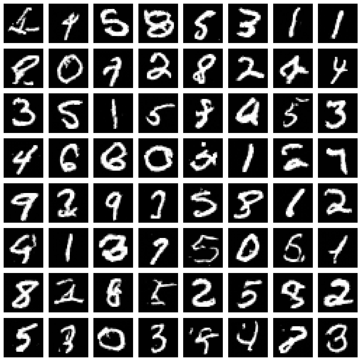
sample_and_visualize
采样一堆图片，然后列表展示
就很简单，非常简单
指定设备、加载权重，把噪声往网络里一丢，完事了？？
就是加了一个反归一化，让输出在一定范围内，然后可视化

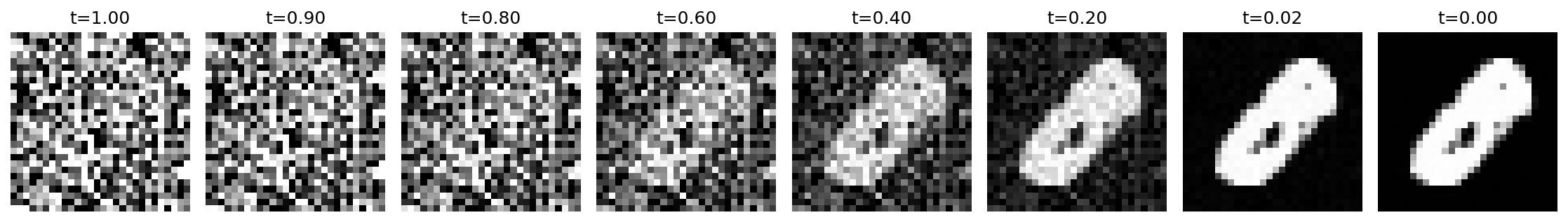
sample_with_progress
单图多步骤采样
也是，指定设备，指定步长，然后丢给神经网络，完事了
最后可视化
就这么简单，优雅

最后是训练用的train.py

import torch
import torch.nn as nn
import torch.optim as optim
from torch.utils.data import DataLoader
from torchvision import datasets, transforms
import matplotlib.pyplot as plt

# 假设你在 ddpm_model.py 中已经添加了 FlowMatchingProcess 类
# 如果没有，请参考上一条回复中的代码添加到 ddpm_model.py
from ddpm_model import SimpleUNet, FlowMatchingProcess


def train_flow_matching(
    num_epochs=100,  # Flow Matching 收敛通常更快，可以适当减少 epoch
    batch_size=128,
    learning_rate=1e-4,  # 建议稍微降低一点 LR，或者保持 2e-4 也可以
    device='cuda' if torch.cuda.is_available() else 'cpu'
):
    """训练 Flow Matching 模型生成 MNIST 数字"""
    print(f"使用设备: {device}")

    # 1. 数据预处理
    # 保持不变：归一化到 [-1, 1]
    transform = transforms.Compose([
        transforms.ToTensor(),
        transforms.Normalize((0.5,), (0.5,))
    ])

    # 加载 MNIST 数据集
    print("加载 MNIST 数据集...")
    train_dataset = datasets.MNIST(
        root='./data',
        train=True,
        download=True,
        transform=transform
    )
    train_loader = DataLoader(
        train_dataset,
        batch_size=batch_size,
        shuffle=True,
        num_workers=2
    )

    # 2. 创建模型和 Flow Matching 过程
    # 模型结构复用 SimpleUNet，参数无需修改
    model = SimpleUNet(image_size=28, in_channels=1,
                       time_emb_dim=32).to(device)

    # 实例化 Flow Matching 处理器
    # 注意：这里不再需要 num_timesteps 参数，因为时间是连续的 [0, 1]
    flow = FlowMatchingProcess(device=device)

    # 优化器
    optimizer = optim.AdamW(model.parameters(), lr=learning_rate)
    criterion = nn.MSELoss()

    # 训练循环
    print("开始 Flow Matching 训练...")
    losses = []

    for epoch in range(num_epochs):
        epoch_loss = 0.0
        num_batches = 0

        for batch_idx, (images, _) in enumerate(train_loader):
            # x_start (也就是 x0, 真实数据)
            x_start = images.to(device)

            # --- Flow Matching 核心逻辑 ---

            # 1. 获取训练元组 (x_t, t, target_v)
            # 这一步替代了 DDPM 中的随机采样 t 和加噪过程
            # flow 内部会自动生成噪声 x1，并计算线性插值 x_t
            x_t, t, target_v = flow.get_train_tuple(x_start)

            # 2. 模型预测
            # 输入：当前插值状态 x_t, 时间 t
            # 输出：预测的速度场 v_pred (意图去拟合 target_v)
            pred_v = model(x_t, t)

            # 3. 计算损失
            # 我们希望模型预测的速度 v_pred 尽可能接近真实方向 (x1 - x0)
            loss = criterion(pred_v, target_v)

            # ---------------------------

            # 反向传播
            optimizer.zero_grad()
            loss.backward()
            # 梯度裁剪 (保持这个好习惯)
            torch.nn.utils.clip_grad_norm_(model.parameters(), 1.0)
            optimizer.step()

            epoch_loss += loss.item()
            num_batches += 1

            if batch_idx % 100 == 0:
                print(
                    f"Epoch [{epoch+1}/{num_epochs}], Batch [{batch_idx}/{len(train_loader)}], Loss: {loss.item():.6f}")

        avg_loss = epoch_loss / num_batches
        losses.append(avg_loss)

        print(f"Epoch [{epoch+1}/{num_epochs}], 平均损失: {avg_loss:.6f}")

        # 每10个epoch保存一次模型
        if (epoch + 1) % 10 == 0:
            torch.save(model.state_dict(), f'fm_mnist_epoch_{epoch+1}.pth')
            print(f"模型已保存到 fm_mnist_epoch_{epoch+1}.pth")

    # 保存最终模型
    torch.save(model.state_dict(), 'fm_mnist_final.pth')
    print("最终模型已保存到 fm_mnist_final.pth")

    # 绘制损失曲线
    plt.figure(figsize=(10, 6))
    plt.plot(losses)
    plt.xlabel('Epoch')
    plt.ylabel('Loss (MSE between v_pred and x1-x0)')
    plt.title('Flow Matching Training Loss')
    plt.grid(True)
    plt.savefig('fm_training_loss.png')
    print("损失曲线已保存到 fm_training_loss.png")

    return model


if __name__ == '__main__':
    # Flow Matching 通常可以用更少的 epoch 达到相同的效果
    model = train_flow_matching(
        num_epochs=100,
        batch_size=128,
        learning_rate=1e-4
    )

训练依旧是一大堆优化器啊啥的，我没有细看，也就步详细展开了

3.Q&A

Q1：盆老师，说是流匹配训练了一个向量场，那为什么在去噪的时候还是简单的减去呢

x = x - v_pred * dt#这不还是把噪声减去吗

A1：这就是流匹配的高明之处了，减去噪声是一个表象，可以看作是高维空间的投影。对于MNIST数据集，可以把每个输入都看作28*28维度的一个点（时间不算在内是因为已经把时间编码加到输入上了），之后，流匹配指导的是这样一个高维空间的点的“移动”，体现出来，就是各个像素点有不同的变化，也就是加减一个噪声。

4.对比扩散模型与流匹配

首先，最直观的感受就是：流匹配太简洁了，形式与理论高度统一，代码简洁易懂不需要数学推导

其次，是去噪的过程。

形象的比喻是：扩散模型要倒着走，一点一点猜上一步的脚印，然后倒退回起点，所以很慢，并且路径可能非常曲折。

流匹配是直接知道了目标，大步流星往回退，非常快。

之后是学习内容。

扩散模型学习的是噪声分布，这一步应该去除哪里的噪声，下一步应该去除哪里的噪声

流匹配学习的是高维的向量场，高维点应该往哪里去，带着整体移动，表现为减去噪声。

所以，流匹配之于扩散模型，就像是扩散模型之于Pixel RNN，这回真是降维打击了。

5.写在最后

流匹配算是最近看的比较舒服的理论了，因为不需要数学推导因为它的代码和理论高度统一，而且极度直观。怪不得pi0和其他VLA都在使用流匹配进行策略或者奖励函数的生成。我想起了考研方浩的名言：高山看海。从更高维度看问题，直接秒杀

（完）