
[学习笔记]DDPM图片降噪
之前学习了一下流匹配的最简单的demo,前两天学长讲了一下扩散模型的简单应用,就尽快学一下然后把博客写上来。
先贴一下仓库
然后是学长的博客
生成扩散模型漫谈(一):DDPM = 拆楼 + 建楼 - 科学空间|Scientific Spaces
代码也是由学长提供的,强无敌的学长
(一个看起来无比古老的博客)
那么接下来,进入正题,开始打这个boss——扩散模型
0.什么是扩散模型
学长的一个比喻非常形象:拆楼与盖楼。
训练的过程就是把楼给拆了
生成的过程就是把楼搭好喽
这里的拆楼,就是在清晰的图片上加噪声
这里的搭楼,就是把雪花图上的噪声消除。
至于为什么叫扩散,因为它的过程很像把一滴墨滴到水中,扩散完的灰色墨水往回逆推。
反正我觉得这个名字还是比较形象的。
1.扩散模型的理论基础
这个部分学长的博客里讲得非常明白,大概就是利用高斯分布的叠加性。至于没法通过观测获得的那些量,那就利用强大的神经网络来进行拟合。
其次,这大概是我第一次真正接触到U-Net这个东西,本来它只存在于人工智能与机器视觉的课堂上,这下它真的走到了工程里
U-Net形如其名,网络像一个U形,因为直接添加了从浅层到深层的连接。
众所周知,深层的网络会包含更加复杂的特征,感受野较大但无法注意到细节;
浅层的网络会注意到一些细节的信息,比如边缘、角点之类
如果直接用MLP一路算下去,就算还原了图片也只能看到一个平滑的光杆(笑
U-Net开辟了一条直接从浅层网络指向深层网络的路径,很好地解决了这个问题。
实现方法:


1 # 上采样(带跳跃连接)
2         x = self.up1(torch.cat([x, x3], dim=1), t)  # [B, 128, 14, 14]
3         # cat:连接矩阵,dim=1表示按列连接,dim=0表示按行连接
4         # 拼接特征,达到连接的效果
5         x = self.up2(torch.cat([x, x2], dim=1), t)  # [B, 64, 28, 28]
6         x = self.up3(torch.cat([x, x1], dim=1), t)  # [B, 64, 28, 28]
也是比较直白。
2.扩散模型的实现方法
还是直接贴代码吧,我感觉注释挺详细了。
不过扩散模型的数学基础有点小复杂,跟代码对应起来有点困难。
不过基本上都是按照数学推导一步一步来的
ddpm_model.py:
  1 import torch
  2 import torch.nn as nn
  3 import math
  4
  5
  6 class SinusoidalPositionalEmbedding(nn.Module):
  7     """时间步的位置编码"""
  8     # 具有线性性质,并且不重复
  9
 10     def __init__(self, dim):
 11         super().__init__()
 12         self.dim = dim
 13
 14     def forward(self, time):
 15         device = time.device  # 获取张量所在的设备,gpu计算步骤
 16         half_dim = self.dim // 2
 17         emb = math.log(10000) / (half_dim - 1)
 18         emb = torch.exp(torch.arange(
 19             half_dim, device=device, dtype=torch.float32) * -emb)
 20         emb = time[:, None].float() * emb[None, :]
 21         emb = torch.cat([emb.sin(), emb.cos()], dim=-1)
 22         return emb
 23
 24
 25 class Block(nn.Module):
 26     """U-Net的基础块"""
 27
 28     def __init__(self, in_ch, out_ch, time_emb_dim, up=False, down=False):
 29         super().__init__()
 30         self.time_mlp = nn.Linear(time_emb_dim, out_ch)  # 简单的线性全连接层
 31         if up:  # U-Net,上下采样
 32             self.conv = nn.ConvTranspose2d(in_ch, out_ch, 4, 2, 1)  # 转置卷积
 33         elif down:
 34             # stride=2 for downsampling
 35             # 简单的卷积层,in out kernel_size stride padding
 36             self.conv = nn.Conv2d(in_ch, out_ch, 3, 2, 1)
 37         else:
 38             self.conv = nn.Conv2d(in_ch, out_ch, 3, padding=1)
 39         self.norm = nn.GroupNorm(8, out_ch)  # 组归一化,总之就是归一化,作用差不多
 40         self.act = nn.SiLU()  # sigmoid,你终于出现了
 41
 42     def forward(self, x, t):
 43         # 时间嵌入
 44         t_emb = self.time_mlp(t)[:, :, None, None]
 45         # 卷积
 46         h = self.conv(x)
 47         # 添加时间嵌入
 48         h = h + t_emb
 49         # 妙哉时间嵌入
 50         # 时间条件注入:通过广播加法,给整张图打上“时间底色”。
 51         # 这不是覆盖特征,而是调节特征,让模型根据当前的时间步 t 来处理图像。
 52
 53         # 归一化和激活
 54         h = self.norm(h)
 55         h = self.act(h)
 56         return h
 57
 58
 59 class SimpleUNet(nn.Module):
 60     """简单的U-Net架构用于DDPM"""
 61
 62     def __init__(self, image_size=28, in_channels=1, time_emb_dim=32):
 63         super().__init__()
 64         self.time_emb_dim = time_emb_dim
 65
 66         # 时间嵌入
 67         self.time_mlp = nn.Sequential(  # 时间嵌入层:使用 nn.Sequential 封装成一个线性流水线
 68             # 作用:将标量时间步 t 转化为高维向量,经过位置编码 -> 线性变换 -> 激活 -> 线性变换
 69             SinusoidalPositionalEmbedding(time_emb_dim),
 70             nn.Linear(time_emb_dim, time_emb_dim),
 71             nn.SiLU(),
 72             nn.Linear(time_emb_dim, time_emb_dim)
 73         )
 74
 75         # 下采样路径
 76         self.down1 = Block(in_channels, 64, time_emb_dim)
 77         self.down2 = Block(64, 128, time_emb_dim, down=True)
 78         self.down3 = Block(128, 256, time_emb_dim, down=True)
 79
 80         # 中间层
 81         self.mid1 = Block(256, 256, time_emb_dim)
 82         self.mid2 = Block(256, 256, time_emb_dim)
 83         # 中间层 (Bottleneck):
 84         # 在最低分辨率(7x7)和最高通道数(256)下处理图像的全局语义信息。
 85         # 这里是连接编码器(Encoder)和解码器(Decoder)的桥梁,负责对提取的深层特征进行转换。
 86
 87         # 上采样路径
 88         self.up1 = Block(256 + 256, 128, time_emb_dim, up=True)  # 7x7 -> 14x14
 89         self.up2 = Block(128 + 128, 64, time_emb_dim,
 90                          up=True)  # 14x14 -> 28x28
 91         # 28x28 -> 28x28 (不再上采样)
 92         self.up3 = Block(64 + 64, 64, time_emb_dim, up=False)
 93
 94         # 输出层
 95         self.out = nn.Conv2d(64, in_channels, 1)
 96
 97     def forward(self, x, timestep):
 98         """
 99         x: [B, C, H, W] 噪声图像
100         timestep: [B] 时间步
101         """
102         # 时间嵌入
103         t = self.time_mlp(timestep)
104
105         # 下采样
106         x1 = self.down1(x, t)  # [B, 64, 28, 28]
107         x2 = self.down2(x1, t)  # [B, 128, 14, 14]
108         x3 = self.down3(x2, t)  # [B, 256, 7, 7]
109
110         # 中间层
111         x = self.mid1(x3, t)
112         x = self.mid2(x, t)
113
114         # 上采样(带跳跃连接)
115         x = self.up1(torch.cat([x, x3], dim=1), t)  # [B, 128, 14, 14]
116         # cat:连接矩阵,dim=1表示按列连接,dim=0表示按行连接
117         x = self.up2(torch.cat([x, x2], dim=1), t)  # [B, 64, 28, 28]
118         x = self.up3(torch.cat([x, x1], dim=1), t)  # [B, 64, 28, 28]
119
120         # 输出
121         return self.out(x)
122
123
124 class DiffusionProcess:
125     """扩散过程"""
126
127     def __init__(self, num_timesteps=1000, beta_start=0.0001, beta_end=0.02, device='cuda'):
128         # num_timesteps: 扩散步数
129         # beta_start: beta的起始值
130         # beta_end: beta的结束值
131         self.num_timesteps = num_timesteps
132         self.device = device
133
134         # 线性beta调度
135         self.betas = torch.linspace(
136             beta_start, beta_end, num_timesteps, device=device)
137         # torch.linspace:生成一个等差数列,线性插值
138         self.alphas = 1.0 - self.betas  # 保留多少原图信息,alpha=1-beta
139
140         self.alphas_cumprod = torch.cumprod(self.alphas, dim=0)
141         # torch.cumprod:计算一个张量的累积积
142         # 对于输入张量 x,输出 y 的第 i 个元素为:
143         # # y[i] = x[0] × x[1] × ... × x[i]
144         self.alphas_cumprod_prev = torch.cat(
145             [torch.tensor([1.0], device=device), self.alphas_cumprod[:-1]])
146         # t-1 的alphas_cumprod
147
148         # 用于采样的参数
149         self.sqrt_alphas_cumprod = torch.sqrt(self.alphas_cumprod)
150         self.sqrt_one_minus_alphas_cumprod = torch.sqrt(
151             1.0 - self.alphas_cumprod)
152         # sqrt(1-alphas_cumprod),数学这一块
153
154         # 用于去噪的参数
155         self.posterior_variance = self.betas * \
156             (1.0 - self.alphas_cumprod_prev) / (1.0 - self.alphas_cumprod)
157
158     def q_sample(self, x_start, t, noise=None):
159         """前向扩散过程:添加噪声"""
160         # x_start: 原始图像
161         if noise is None:
162             noise = torch.randn_like(x_start)
163             # randn_like:生成一个与给定张量相同形状的随机张量,并使用给定张量的数据类型和设备,正态分布
164
165         sqrt_alphas_cumprod_t = self.sqrt_alphas_cumprod[t].view(-1, 1, 1, 1)
166         sqrt_one_minus_alphas_cumprod_t = self.sqrt_one_minus_alphas_cumprod[t].view(
167             -1, 1, 1, 1)
168
169         return sqrt_alphas_cumprod_t * x_start + sqrt_one_minus_alphas_cumprod_t * noise
170     # 按照数学模型加噪声
171
172     def p_sample(self, model, x_t, t):
173         """反向去噪过程:单步采样"""
174         # 预测噪声
175         predicted_noise = model(x_t, t)
176
177         # 计算系数
178         alpha_t = self.alphas[t].view(-1, 1, 1, 1)
179         alpha_cumprod_t = self.alphas_cumprod[t].view(-1, 1, 1, 1)
180         beta_t = self.betas[t].view(-1, 1, 1, 1)
181
182         # 计算x_0的预测值
183         pred_x_start = (x_t - torch.sqrt(1.0 - alpha_cumprod_t)
184                         * predicted_noise) / torch.sqrt(alpha_cumprod_t)
185         pred_x_start = torch.clamp(pred_x_start, -1.0, 1.0)
186         # torch.clamp:将张量中的元素限制在给定的区间内
187         # 不同于归一化,更像二值化,将超出范围的值截断为边界值
188         # 先预测一个x0,然后根据这个x0预测x_t,相当于锚点
189
190         # 对于t=0,直接返回预测的x_0
191         if t[0] == 0:
192             return pred_x_start
193
194         # 计算alpha_cumprod_prev
195         alpha_cumprod_prev_t = self.alphas_cumprod_prev[t].view(-1, 1, 1, 1)
196
197         # 后验均值的系数
198         posterior_mean_coef1 = torch.sqrt(
199             alpha_cumprod_prev_t) * beta_t / (1.0 - alpha_cumprod_t)
200         posterior_mean_coef2 = torch.sqrt(
201             alpha_t) * (1.0 - alpha_cumprod_prev_t) / (1.0 - alpha_cumprod_t)
202
203         # 计算后验均值
204         posterior_mean = posterior_mean_coef1 * \
205             pred_x_start + posterior_mean_coef2 * x_t
206
207         # 计算后验方差
208         posterior_variance = self.posterior_variance[t].view(-1, 1, 1, 1)
209
210         # 采样
211         noise = torch.randn_like(x_t)
212         # 叠加噪声,补充细节:把“平均的模糊”变成“具体的纹理”
213         return posterior_mean + torch.sqrt(posterior_variance) * noise
214
215     def p_sample_loop(self, model, shape, num_samples=1):
216         """完整的反向采样过程"""
217         model.eval()
218         with torch.no_grad():
219             # 从纯噪声开始
220             x = torch.randn(num_samples, *shape, device=self.device)
221             # torch.randn:生成一个张量,张量的元素从标准正态分布中随机采样
222
223             # 逐步去噪
224             for i in reversed(range(self.num_timesteps)):
225                 # reversed:返回一个迭代器,迭代器返回列表或元组中的元素,按从后到前的顺序
226                 t = torch.full((num_samples,), i,
227                                device=self.device, dtype=torch.long)
228                 # torch.full:生成一个张量,张量的元素填充为给定值
229                 # torch.long:表示整数
230                 x = self.p_sample(model, x, t)
231                 # 丢进神经网络,统统丢进神经网络!
232
233         model.train()
234         return x
这个模块定义了U-Net、扩散过程
简单介绍一下各个模块:
class SinusoidalPositionalEmbedding(nn.Module):
这个class在forward里定义了一个时间编码器,总之就是把时间步嵌入到向量里,告诉流匹配模型当前到哪个时间步了
class Block(nn.Module):
这个类定义了U-Net网络的基本构成,U-Net由多个略有不同的Block组成
首先是init,定义了各个层
其次是forward,加入了时间嵌入
class SimpleUNet(nn.Module):
这个类具体实现了U-Net
在Block前,又增加了一些层,一些时间嵌入啊、sigmoid啊、线性层之类的
接着就是具体的采样过程了
class DiffusionProcess:
这个类是整个扩散过程与逆扩散过程的实现
在init中,计算了一些后续要用到的量以便查表(比如数学推导中用到的乘法前缀和,以便查表)
q_sample函数即向清晰的图像中加噪声,不同的时间步有不同的噪声量
p_sample即单步去噪过程
p_sample_loop即多次使用单步降噪,获得最终图片
这个文件大概就是这样
接下来是sample.py
  1 import torch
  2 import numpy as np
  3 import matplotlib.pyplot as plt
  4 from ddpm_model import SimpleUNet, DiffusionProcess
  5
  6
  7 def sample_and_visualize(
  8     model_path='ddpm_mnist_final.pth',
  9     num_samples=16,
 10     num_timesteps=1000,
 11     device='cuda' if torch.cuda.is_available() else 'cpu',
 12     save_path='generated_samples.png'
 13 ):
 14     """从训练好的模型采样并可视化"""
 15     print(f"使用设备: {device}")
 16
 17     # 加载模型
 18     model = SimpleUNet(image_size=28, in_channels=1,
 19                        time_emb_dim=32).to(device)
 20     model.load_state_dict(torch.load(model_path, map_location=device))
 21     model.eval()
 22     # 网络初始化
 23
 24     # 创建扩散过程
 25     diffusion = DiffusionProcess(num_timesteps=num_timesteps, device=device)
 26
 27     print(f"生成 {num_samples} 个样本...")
 28
 29     # 采样
 30     samples = diffusion.p_sample_loop(
 31         model, shape=(1, 28, 28), num_samples=num_samples)
 32     # 去噪过程
 33     samples = samples.cpu()
 34     # 把数据搬运到cpu上
 35
 36     # 反归一化:从[-1, 1]回到[0, 1]
 37     samples = (samples + 1.0) / 2.0
 38     samples = torch.clamp(samples, 0.0, 1.0)
 39     # 先归一化,再截断
 40
 41     # 可视化
 42     grid_size = int(np.sqrt(num_samples))
 43     fig, axes = plt.subplots(grid_size, grid_size, figsize=(10, 10))
 44     axes = axes.flatten()
 45
 46     for i in range(num_samples):
 47         img = samples[i].squeeze().numpy()
 48         axes[i].imshow(img, cmap='gray')
 49         axes[i].axis('off')
 50
 51     plt.tight_layout()
 52     plt.savefig(save_path, dpi=150, bbox_inches='tight')
 53     print(f"生成的样本已保存到 {save_path}")
 54
 55     return samples
 56
 57
 58 def sample_with_progress(
 59     model_path='ddpm_mnist_final.pth',
 60     num_samples=16,
 61     num_timesteps=1000,
 62     device='cuda' if torch.cuda.is_available() else 'cpu',
 63     save_path='generation_progress.png'
 64 ):
 65     """可视化生成过程(中间步骤)"""
 66     print(f"使用设备: {device}")
 67
 68     # 加载模型
 69     model = SimpleUNet(image_size=28, in_channels=1,
 70                        time_emb_dim=32).to(device)
 71     model.load_state_dict(torch.load(model_path, map_location=device))
 72     model.eval()
 73
 74     # 创建扩散过程
 75     diffusion = DiffusionProcess(num_timesteps=num_timesteps, device=device)
 76
 77     # 从纯噪声开始
 78     x = torch.randn(1, 1, 28, 28, device=device)
 79
 80     # 选择要可视化的时间步
 81     timesteps_to_show = [999, 800, 600, 400, 200, 100, 50, 0]
 82     images = []
 83
 84     with torch.no_grad():
 85         for i in reversed(range(num_timesteps)):
 86             t = torch.full((1,), i, device=device, dtype=torch.long)
 87             x = diffusion.p_sample(model, x, t)
 88
 89             if i in timesteps_to_show:
 90                 img = x.cpu().squeeze().numpy()
 91                 img = (img + 1.0) / 2.0
 92                 img = np.clip(img, 0.0, 1.0)
 93                 images.append((i, img))
 94
 95     # 可视化生成过程
 96     fig, axes = plt.subplots(1, len(images), figsize=(15, 3))
 97     for idx, (t, img) in enumerate(images):
 98         axes[idx].imshow(img, cmap='gray')
 99         axes[idx].set_title(f't={t}')
100         axes[idx].axis('off')
101
102     plt.tight_layout()
103     plt.savefig(save_path, dpi=150, bbox_inches='tight')
104     print(f"生成过程已保存到 {save_path}")
105
106
107 if __name__ == '__main__':
108     # 生成样本
109     samples = sample_and_visualize(
110         model_path='ddpm_mnist_final.pth',
111         num_samples=64,
112         save_path='generated_samples.png'
113     )
114
115     # 可视化生成过程
116     sample_with_progress(
117         model_path='ddpm_mnist_final.pth',
118         save_path='generation_progress.png'
119     )
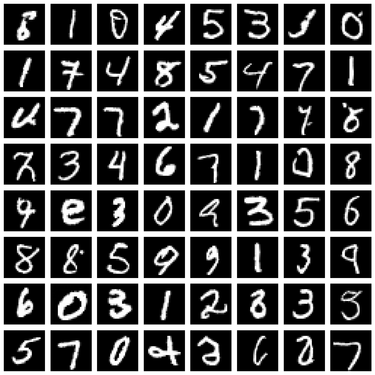
def sample_and_visualize
这个函数生成了一批图片,然后一起降噪,并可视化为一个表格(图1所示)
加载模型,生成样本,扩散!
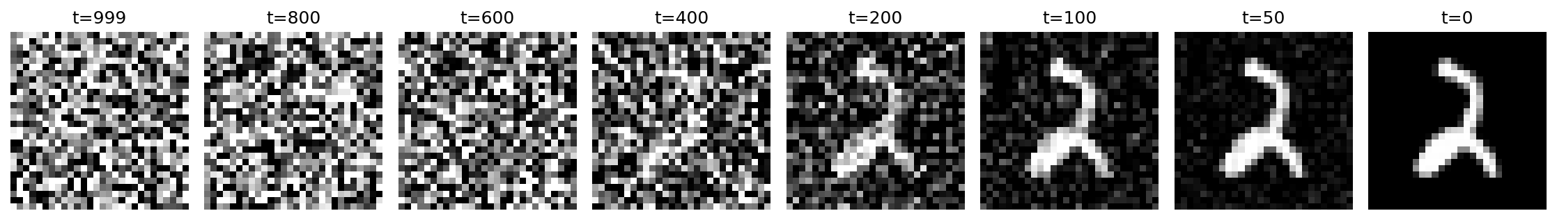
def sample_with_progress
这个函数生成了一张图片,把降噪过程展示了出来(图2所示)
加载模型,生成样本,扩散!
接下来是train.py(其实就没什么好看的了)
  1 import torch
  2 import torch.nn as nn
  3 import torch.optim as optim
  4 from torch.utils.data import DataLoader
  5 from torchvision import datasets, transforms
  6 import matplotlib.pyplot as plt
  7 from ddpm_model import SimpleUNet, DiffusionProcess
  8
  9
 10 def train_ddpm(
 11     num_epochs=500,
 12     batch_size=128,
 13     learning_rate=2e-4,
 14     num_timesteps=1000,
 15     device='cuda' if torch.cuda.is_available() else 'cpu'
 16 ):
 17     """训练DDPM模型生成MNIST数字"""
 18     print(f"使用设备: {device}")
 19
 20     # 数据预处理:归一化到[-1, 1]
 21     transform = transforms.Compose([
 22         transforms.ToTensor(),
 23         transforms.Normalize((0.5,), (0.5,))  # 从[0,1]归一化到[-1,1]
 24     ])
 25
 26     # 加载MNIST数据集
 27     print("加载MNIST数据集...")
 28     train_dataset = datasets.MNIST(
 29         root='./data',
 30         train=True,
 31         download=True,
 32         transform=transform
 33     )
 34     train_loader = DataLoader(
 35         train_dataset,
 36         batch_size=batch_size,
 37         shuffle=True,
 38         num_workers=2
 39     )
 40
 41     # 创建模型和扩散过程
 42     model = SimpleUNet(image_size=28, in_channels=1, time_emb_dim=32).to(device)
 43     diffusion = DiffusionProcess(num_timesteps=num_timesteps, device=device)
 44
 45     # 优化器
 46     optimizer = optim.AdamW(model.parameters(), lr=learning_rate)
 47     criterion = nn.MSELoss()
 48
 49     # 训练循环
 50     print("开始训练...")
 51     losses = []
 52
 53     for epoch in range(num_epochs):
 54         epoch_loss = 0.0
 55         num_batches = 0
 56
 57         for batch_idx, (images, _) in enumerate(train_loader):
 58             images = images.to(device)
 59
 60             # 随机采样时间步
 61             t = torch.randint(0, num_timesteps, (images.shape[0],), device=device)
 62
 63             # 采样噪声
 64             noise = torch.randn_like(images)
 65
 66             # 前向扩散:添加噪声
 67             x_t = diffusion.q_sample(images, t, noise)
 68
 69             # 预测噪声
 70             predicted_noise = model(x_t, t)
 71
 72             # 计算损失
 73             loss = criterion(predicted_noise, noise)
 74
 75             # 反向传播
 76             optimizer.zero_grad()
 77             loss.backward()
 78             # 梯度裁剪
 79             torch.nn.utils.clip_grad_norm_(model.parameters(), 1.0)
 80             optimizer.step()
 81
 82             epoch_loss += loss.item()
 83             num_batches += 1
 84
 85             if batch_idx % 100 == 0:
 86                 print(f"Epoch [{epoch+1}/{num_epochs}], Batch [{batch_idx}/{len(train_loader)}], Loss: {loss.item():.6f}")
 87
 88         avg_loss = epoch_loss / num_batches
 89         losses.append(avg_loss)
 90
 91         print(f"Epoch [{epoch+1}/{num_epochs}], 平均损失: {avg_loss:.6f}")
 92
 93         # 每10个epoch保存一次模型
 94         if (epoch + 1) % 10 == 0:
 95             torch.save(model.state_dict(), f'ddpm_mnist_epoch_{epoch+1}.pth')
 96             print(f"模型已保存到 ddpm_mnist_epoch_{epoch+1}.pth")
 97
 98     # 保存最终模型
 99     torch.save(model.state_dict(), 'ddpm_mnist_final.pth')
100     print("最终模型已保存到 ddpm_mnist_final.pth")
101
102     # 绘制损失曲线
103     plt.figure(figsize=(10, 6))
104     plt.plot(losses)
105     plt.xlabel('Epoch')
106     plt.ylabel('Loss')
107     plt.title('Training Loss')
108     plt.grid(True)
109     plt.savefig('training_loss.png')
110     print("损失曲线已保存到 training_loss.png")
111
112     return model, diffusion
113
114
115 if __name__ == '__main__':
116     model, diffusion = train_ddpm(
117         num_epochs=500,
118         batch_size=128,
119         learning_rate=2e-4,
120         num_timesteps=1000
121     )
3.Q&A
列一些我学习过程中遇到的比较神奇的问题吧,记录一下,也希望能够帮助到一些人入门(坑)
感谢gemini的大力支持没有gemini我死这了
Q1:为什么时间码与前向传播的特征直接就相加了?这样不会导致特征消融或是时间码重复吗?比如两个不同的图片,加上不同的时间码反而相同了?
A1:应该不会,这个时间码更像一种“偏置”,即将整个图片的像素都“变亮”或者“变暗”了固定值。当然,这里是对于提取出的特征的偏执,所以不仅不会重复,还利于广播(反正我是似懂非懂的)
Q2:为什么在单步去噪过程中要直接预测一个x0(即初始图像)呢?
A2:在数学推导里有出现x0,但是我们不知道真正的x0,所以只能用现阶段的模型预测一个,不管它有多离谱,先用着,有比没有强,当作一个锚点来进行指导(依旧似懂非懂,反正工程上存在肯定有它的好处就对了)
翻了一下对着gemini哈气的界面,暂时就找到这两个。那大概就写到这吧
(完)

 浙公网安备 33010602011771号