DeepLearning - Regularization

I have finished the first course in the DeepLearnin.ai series. The assignment is relatively easy, but it indeed provides many interesting insight. You can find some summary notes of the first course in my previous 2 posts.

• sigmoid and shallow NN
• Forward and Backward propogation

Now let's move on to the second course - Improving Deep Neural Networks: Hyper-parameter tuning, Regularization and Optimization..The second course mainly focus on some details in model tuning, including regularization, Batch, optimization, and some other techniques. Let's start with regularization.

Regularization is used to fight model over fitting. Almost all the model over fits to some extent. Because the distribution of your train and test set can't be exactly the same. Meaning your model will always learn something unique to your training set. That's why we need regularization. It tries to make your model more generalize without sacrificing too much performance- the trade off between bias (Performance) and variance (Generalization)

Any feedback is welcomed. And please correct me if I got anything wrong.

1. Parameter Regularization - L2

L2 regularization is a popular method outside NN. It is frequently used in regression, random forest and etc. With L2 regularization, the loss function of NN will be following:

\[\tilde{L}(a, y) = L(a, y) + \frac{\alpha}{2} \|w \|^2_2 \]

For layer L, above regularization term can be calculated as following:

\[\|w^{[L]} \|^2_2 = \sum^{n^{[L-1]}}_{i=1}\sum^{n^{[L]}}_{j=1} w_{ij}^2 \]

But why can adding L2 regularization help reduces over-fitting? We can get a rough idea of this from another name of it - weight Decay. Basically L2 works by pushing the weight close to 0. It is more obvious from gradient descent:

\[\frac{\partial\tilde{L}(a,y)}{\partial w} = \frac{\partial L(a,y)}{\partial w} +\alpha{w} \]

\[w \leftarrow w - \epsilon{(\frac{\partial L(a,y)}{\partial w} +\alpha{w})} \]

Further clean it up, we will get following:

\[w \leftarrow (1- \epsilon\alpha)w - \epsilon{\frac{\partial L(a,y)}{\partial w} } \]

Compare with the original gradient, we can see after L2 regularization, parameter \(w\) will shrink by \((1- \alpha\epsilon)\) in each iteration.

So far I don't know whether you have the same confusion like me. Why would shrinking weight helps in reduce over-fitting? I found 2 ways to convince myself. Let's go with the intuition one first.

(1). Some intuition into weight decay

Andrew gives the below intuition, which is simple but very convincing. Below is Tanh function, it is frequently used as activation function in the hidden layer.

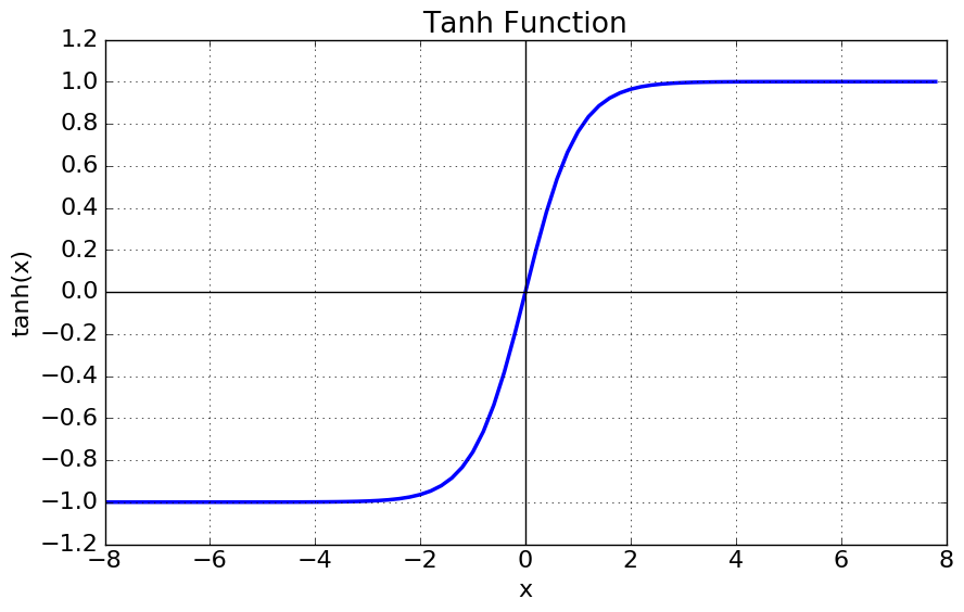
We can see when the function is around 0. it is almost linear. The non-linearity is more significant when the X gets bigger. Mean By pushing the weight close to 0, we will get a activation function with less non-linearity. Therefore weight decay can lead to a less complicated model and less over-fitting.

(2). Some math of weight decay

Of course, we can also prove the effect of **weight decay mathematically.

Let's use \(w^*\) to denote the optimal weight for original model without regularization. \(w^* = argmin_w{L(a, y)}\)
\(H\) is the Hessian matrix at \(w^*\), where \(H_{ij} = \frac{\partial^2L}{\partial{w_i}\partial{w_j}}\)
\(J\) is the Jacobian matrix at \(w^*\), where \(J_{j} = \frac{\partial{L}}{\partial{w_i}}\)
We can use Taylor rule to get the approximate form of the new loss function.

\[\tilde{L}(w) = L(w^*) + J(w- w^*) + \frac{1}{2}(w-w^*)^TH(w-w^*) + \frac{\alpha}{2} \|w \|^2_2 \]

Because \(w^*\) is at optimzal, so \(J=0\) and \(H\) is positive. So above can be simplified as below

\[\tilde{L}(w) = L(w^*) + \frac{1}{2}(w-w^*)^TH(w-w^*) + \frac{\alpha}{2} \|w \|^2_2 \]

The new gradient \(\tilde{w}\) is following

\[\frac{\partial{\tilde{L}}}{\partial{w}} = H(\tilde{w}-w^*) + \alpha{\tilde{w}}= 0 \]

And we will get the new optimal:

\[\tilde{w} = (H + \alpha{I})^{-1}w^* \]

Because H is positive matrix, so we can decompose H into \(H = Q\Lambda{Q^T}\). where \(\Lambda\) is interpreted as the importance of weight \(w\). So above form will be following:

\[\tilde{w} = Q(\Lambda + \alpha{I})^{-1} Q^T w^* \]

Each weight \(w_i\) is scaled by \(\frac{\lambda_i}{\lambda_i+\alpha}\). If \(w_i\) is bigger, regularization will has less impact. Basically L2 shrinks the weight that are not important to the model.

2. Dropout

Dropout is a very simple, yet very powerful technique in regularization. It functions by randomly assigning 0 to neuron in hidden layer. It can be easily understood using following code:

import numpy as np 
drop = np.random.rand(a.shape) < keep_probs ## drop out rate 
a = np.multiply(drop,a ) ## randomly turned off neuron 

when keep_probs gets lower, more neuron will be shut down. And here is a few ways to understand why dropout can reduce overfitting

(1). Intuition 1 - spread out weight

One way to understand dropout is that it helps spread out the weights across neurons in each hidden layer.

It is possible that the original model has higher weight on a few neurons and much lower weight on others. With dropout, the lower weighted neruon will have relatively higher weight.

Simiilar method is also used in Random Forest. In each iteraion, we randomly select a subset of columns to build the tree, so that the less importan column will have higher probably to got picked.

(2). Intuition 2 - Bagging

Bagging(Bootstrap aggregating) is used to reduce the variance of model by averaging across several models. It is very popularly used in Kaggle competition. A lot of 1st rank model is actually an average of several models.

Just like investing in portfolio is generally less risky than investing in one asset. Because the asset themselves are not entirely correlated. Therefore the variance of portfolio is smaller than the sum of the variance from each asset.

To some extent, dropout is also bagging. It randomly shuts down neurons through forward propogation, leading to a slightly different neural netwrok in each iteration (sub neural network).

The difference is in bagging, all the models are independent, while using dropout, all the sub neural networks share all the parameters. And we can view the final neural network as an aggregation of all the sub neural networks.

(3). Intuition 3 - Noise injection

Dropout also can be viewed as injecting noise into the hidden layer.
It multiplies the original hidden neuron by a randomly generated indicator (0/1). Multiplicative noise is sometimes regarded as better than additive noise. Because for additive noise, the model can easily reverse it by giving bigger weight to make the added noise less significant.

3. Early Stopping

This technique is wildly used, because it is very easy to implement and very efficient. You just need to stop training after certain threshold - a hyper parameter to train.

The best part of this method is that it doesn't change anything in the model training. And it can be easily combined with other method.

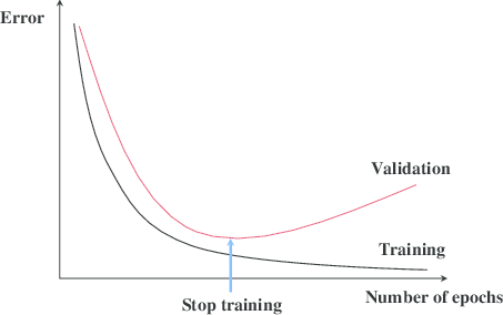
Because final goal of the model is to have better performance on the test set. So the stopping threshold is set on the validation set. Basically we should stop the model when the validation error stops decreasing after N iteration, like following:

4. other methods

There are many other techniques like data augmentation, noise robustness, multi-task learning. They are mainly used at more specific area. We will go through them later.

---

Reference

1. Ian Goodfellow, Yoshua Bengio, Aaron Conrville, "Deep Learning"
2. Deeplearning.ai https://www.deeplearning.ai/