DeepLearning Intro - sigmoid and shallow NN

This is a series of Machine Learning summary note. I will combine the deep learning book with the deeplearning open course . Any feedback is welcomed!

First let's go through some basic NN concept using Bernoulli classification problem as an example.

Activation Function

1.Bernoulli Output

1. Definition

When dealing with Binary classification problem, what activavtion function should we use in the output layer?
Basically given \(x \in R^n\), How to get \(P(y=1|x)\) ?

2. Loss function

Let $\hat{y} = P(y=1|x) $, We would expect following output

\[P(y|x) = \begin{cases} \hat{y} & \quad when & y= 1\\ 1-\hat{y} & \quad when & y= 0\\ \end{cases} \]

Above can be simplified as

\[P(y|x)= \hat{y}^{y}(1-\hat{y})^{1-y} \]

Therefore, the maximum likelihood of m training samples will be

\[\theta_{ML} = argmax\prod^{m}_{i=1}P(y^i|x^i) \]

As ususal we take the log of above function and get following. Actually for gradient descent log has other advantages, which we will discuss later.

\[log(\theta_{ML}) = argmax\sum^{m}_{i=1} ylog(\hat{y})+(1-y)log(1-\hat{y}) \]

And the cost function for optimization is following

\[J(w,b) = \sum ^{m}_{i=1}L(y^i,\hat{y}^i)= -\sum^{m}_{i=1}ylog(\hat{y})+(1-y)log(1-\hat{y}) \]

The cost function is the sum of loss from m training samples, which measures the performance of classification algo.
And yes here it is exactly the negative of log likelihood. While Cost function can be different from negative log likelihood, when we apply regularization. But here let's start with simple version.

So here comes our next problem, how can we get 1-dimension $ log(\hat{y})$, given input \(x\), which is n-dimension vector ?

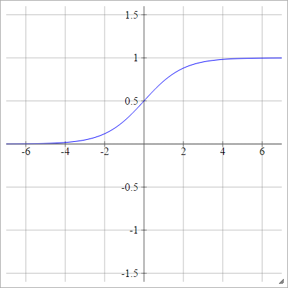
3. Activtion function - Sigmoid

Let \(h\) denotes the output from the previous hidden layer that goes into the final output layer. And a linear transformation is applied to \(h\) before activation function.
Let \(z = w^Th +b\)

The assumption here is

\[log(\hat{y}) = \begin{cases} z & \quad when & y= 1\\ 0 & \quad when & y= 0\\ \end{cases} \]

Above can be simplified as

\[log(\hat{y}) = yz\quad \to \quad \hat{y} = exp(yz) \]

This is an unnormalized distribution of \(\hat{y}\). Because \(y\) denotes probability, we need to further normalize it to $ [0,1]$.

\[\hat{y} = \frac{exp(yz)} {\sum^1_{y=0}exp(yz)} \\ =\frac{exp(z)}{1+exp(z)}\\ \quad \quad \quad \quad = \frac{1}{1+exp(-z)} = \sigma(z) \]

Bingo! Here we go - Sigmoid Function: \(\sigma(z) = \frac{1}{1+exp(-z)}\)

\[p(y|x) = \begin{cases} \sigma(z) & \quad when & y= 1\\ 1-\sigma(z) & \quad when & y= 0\\ \end{cases} \]

Sigmoid function has many pretty cool features like following:

\[ 1- \sigma(x) = \sigma(-x) \\ \frac{d}{dx} \sigma(x) = \sigma(x)(1-\sigma(x)) \\ \quad \quad = \sigma(x)\sigma(-x) \]

Using the first feature above, we can further simply the bernoulli output into following:

\[p(y|x) = \sigma((2y-1)z) \]

4. gradient descent and back propagation

Now we have target cost fucntion to optimize. How does the NN learn from training data? The answer is -- Back Propagation.

Actually back propagation is not some fancy method that is designed for Neural Network. When training sample is big, we can use back propagation to train linear regerssion too.

Back Propogation is iteratively using the partial derivative of cost function to update the parameter, in order to reach local optimum.

$ \
Looping \quad m \quad samples :\
w= w - \frac{\partial J(w,b)}{\partial w} \
b= b - \frac{\partial J(w,b)}{\partial b}
$

Bascically, for each training sample \((x,y)\), we compare the \(y\) with \(\hat{y}\) from output layer. Get the difference, and compute which part of difference is from which parameter( by partial derivative). And then update the parameter accordingly.

And the derivative of sigmoid function can be calcualted using chaining method:
For each training sample, let \(\hat{y}=a = \sigma(z)\)

\[ \frac{\partial L(a,y)}{\partial w} = \frac{\partial L(a,y)}{\partial a} \cdot \frac{\partial a}{\partial z} \cdot \frac{\partial z}{\partial w}\]

Where
1.$\frac{\partial L(a,y)}{\partial a}
=-\frac{y}{a} + \frac{1-y}{1-a} $
Given loss function is
\(L(a,y) = -(ylog(a) + (1-y)log(1-a))\)

2.\(\frac{\partial a}{\partial z} = \sigma(z)(1-\sigma(z)) = a(1-a)\).
See above for sigmoid features.

3.\(\frac{\partial z}{\partial w} = x\)
Put them together we get :

\[\frac{\partial L(a,y)}{\partial w} = (a-y)x \]

This is exactly the update we will have from each training sample \((x,y)\) to the parameter \(w\).

5. Entire work flow.

Summarizing everything. A 1-layer binary classification neural network is trained as following:

• Forward propagation: From \(x\), we calculate \(\hat{y}= \sigma(z)\)
• Calculate the cost function \(J(w,b)\)
• Back propagation: update parameter \((w,b)\) using gradient descent.
• keep doing above until the cost function stop improving (improment < certain threshold)

6. what's next?

When NN has more than 1 layer, there will be hidden layers in between. And to get non-linear transformation of x, we also need different types of activation function for hidden layer.

However sigmoid is rarely used as hidden layer activation function for following reasons

• vanishing gradient descent
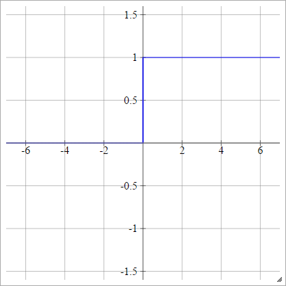
  the reason we can't use [left] as activation function is because the gradient is 0 when \(z>1 ,z <0\).
  Sigmoid only solves this problem partially. Becuase \(gradient \to 0\), when \(z>1 ,z <0\).

\(p(y=1|x)= max\{0,min\{1,z\}\}\)	\(p(y=1|x)= \sigma(z)\)

• non-zero centered

To be continued

---

Reference

1. Ian Goodfellow, Yoshua Bengio, Aaron Conrville, "Deep Learning"
2. Deeplearning.ai https://www.deeplearning.ai/