
DeepLearning - Forard & Backward Propogation
In the previous post I go through basic 1-layer Neural Network with sigmoid activation function, including
-
How to get sigmoid function from a binary classification problem?
-
NN is still an optimization problem, so what's the target to optimize? - cost function
-
How does model learn?- gradient descent
-
Work flow of NN? - Backward/Forward propagation
Now let's get deeper to 2-layers Neural Network, from where you can have as many hidden layers as you want. Also let's try to vectorize everything.
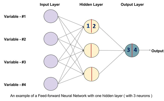
1. The architecture of 2-layers shallow NN
Below is the architecture of 2-layers NN, including input layer, one hidden layer and one output layer. The input layer is not counted.
(1) Forward propagation
In each neuron, there are 2 activities going on after take in the input from previous hidden layer:
- a linear transformation of the input
- a non-linear activation function applied after
Then the ouput will pass to the next hidden layer as input.
From input layer to output layer, do above computation layer by layer is forward propagation. It tries to map each input \(x \in R^n\) to $ y$.
For each training sample, the forward propagation is defined as following:
\(x \in R^{n*1}\) denotes the input data. In the picture n = 4.
\((w^{[1]} \in R^{k*n},b^{[1]}\in R^{k*1})\) is the parameter in the first hidden layer. Here k = 3.
\((w^{[2]} \in R^{1*k},b^{[2]}\in R^{1*1})\) is the parameter in the output layer. The output is a binary variable with 1 dimension.
\((z^{[1]} \in R^{k*1},z^{[2]}\in R^{1*1})\) is the intermediate output after linear transformation in the hidden and output layer.
\((a^{[1]} \in R^{k*1},a^{[2]}\in R^{1*1})\) is the output from each layer. To make it more generalize we can use \(a^{[0]} \in R^n\) to denote \(x\)
*Here we use \(g(x)\) as activation function for hidden layer, and sigmoid \(\sigma(x)\) for output layer. we will discuss what are the available activation functions \(g(x)\) out there in the following post. What happens in forward propagation is following:
\([1]\) \(z^{[1]} = {w^{[1]}} a^{[0]} + b^{[1]}\)
\([2]\) \(a^{[1]} = g((z^{[1]} ) )\)
\([3]\) \(z^{[2]} = {w^{[2]}} a^{[1]} + b^{[2]}\)
\([4]\) \(a^{[2]} = \sigma(z^{[2]} )\)
(2) Backward propagation
After forward propagation, for each training sample \(x\) is done ,we will have a prediction \(\hat{y}\). Comparing \(\hat{y}\) with \(y\), we then use the error between prediction and real value to update the parameter via gradient descent.
Backward propagation is passing the gradient descent from output layer back to input layer using chain rule like below. The deduction is in the previous post.
\([4]\) \(dz^{[2]} = a^{[2]} - y\)
\([3]\) \(dw^{[2]} = dz^{[2]} a^{[1]T}\)
\([3]\) \(db^{[2]} = dz^{[2]}\)
\([2]\) \(dz^{[1]} = da^{[1]} * g^{[1]'}(z[1]) = w^{[2]T} dz^{[2]}* g^{[1]'}(z[1])\)
\([1]\) \(dw^{[1]} = dz^{[1]} a^{[0]T}\)
\([1]\) \(db^{[1]} = dz^{[1]}\)
2. Vectorize and Generalize your NN
Let's derive the vectorize representation of the above forward and backward propagation. The usage of vector is to speed up the computation. We will talk about this again in batch gradient descent.
\(w^{[1]},b^{[1]}, w^{[2]}, b^{[2]}\) stays the same. Generally \(w^{[i]}\) has dimension \((h_{i},h_{i-1})\) and \(b^{[i]}\) has dimension \((h_{i},1)\)
\(Z^{[1]} \in R^{k*m}, Z^{[2]} \in R^{1*m}, A^{[0]} \in R^{n*m}, A^{[1]} \in R^{k*m}, A^{[2]}\in R^{1*m}\) where \(A^{[0]}\)is the input vector, each column is one training sample.
(1) Forward propogation
Follow above logic, vectorize representation is below:
\([1]\) \(Z^{[1]} = {w^{[1]}} A^{[0]} + b^{[1]}\)
\([2]\) \(A^{[1]} = g((Z^{[1]} ) )\)
\([3]\) \(Z^{[2]} = {w^{[2]}} A^{[1]} + b^{[2]}\)
\([4]\) \(A^{[2]} = \sigma(Z^{[2]} )\)
Have you noticed that the dimension above is not a exact matched?
\({w^{[1]}} A^{[0]}\) has dimension \((k,m)\), \(b^{[1]}\) has dimension \((k,1)\).
However Python will take care of this for you with Broadcasting. Basically it will replicate the lower dimension to the higher dimension. Here \(b^{[1]}\) will be replicated m times to become \((k,m)\)
(1) Backward propogation
Same as above, backward propogation will be:
\([4]\) \(dZ^{[2]} = A^{[2]} - Y\)
\([3]\) \(dw^{[2]} =\frac{1}{m} dZ^{[2]} A^{[1]T}\)
\([3]\) \(db^{[2]} = \frac{1}{m} \sum{dZ^{[2]}}\)
\([2]\) \(dZ^{[1]} = dA^{[1]} * g^{[1]'}(z[1]) = w^{[2]T} dZ^{[2]}* g^{[1]'}(z[1])\)
\([1]\) \(dw^{[1]} = \frac{1}{m} dZ^{[1]} A^{[0]T}\)
\([1]\) \(db^{[1]} = \frac{1}{m} \sum{dZ^{[1]} }\)
In the next post, I will talk about some other details in NN, like hyper parameter, activation function.
To be continued.
Reference
- Ian Goodfellow, Yoshua Bengio, Aaron Conrville, "Deep Learning"
- Deeplearning.ai https://www.deeplearning.ai/

 浙公网安备 33010602011771号