A Concise Introduction to Logic - PART III: INDUCTIVE LOGIC - Chapter 11 and Chapter 12

PART III: INDUCTIVE LOGIC

Chapter 11: Probability

11.1 Theories of Probability

Probability is a topic that is central to the question of induction, but like causality, it has different meanings. Consider the following statements:

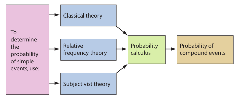
In each statement the word “probability” is used in a different sense. This difference stems from the fact that a different procedure is used in each case to determine or estimate the probability. To determine the probability of picking a spade from a deck of cards, a purely mathematical procedure is used. Given that there are fifty-two cards in a deck and thirteen are spades, thirteen is divided by fifty-two to obtain one-fourth. A different procedure is used to determine the probability that a twenty-year-old man will live to age seventy-five. For this, one must sample a large number of twenty-yearold men and count the number that live fifty-five more years. Yet a different procedure is used to determine the probability that Margaret and Peter will get married. This probability can only be estimated roughly, and doing so requires that we become acquainted with Margaret and Peter and with how they feel toward each other and toward marriage. These three procedures give rise to three distinct theories about probability: the classical theory, the relative frequency theory, and the subjectivist theory.

The classical theory of probability traces its origin to the work of the seventeenthcentury mathematicians Blaise Pascal and Pierre de Fermat in determining the betting odds for a game of chance. The theory is otherwise called the a priori theory of probability because the computations are made independently of any sensory observation of actual events. According to the classical theory, the probability of an event A is given by the formula

where f is the number of favorable outcomes and n is the number of possible outcomes. For example, in computing the probability of drawing an ace from a poker deck, the number of favorable outcomes is four (because there are four aces) and the number of possible outcomes is fifty-two (because there are fifty-two cards in the deck). Thus, the probability of that event is 4/52 or 1/13 (or .077).

It is important not to confuse the probability of an event’s happening with the betting odds of its happening. For events governed by the classical theory, the fair betting odds that an event A will happen is given by the formula

where f is the number of favorable outcomes, and u is the number of unfavorable outcomes. For example, the fair betting odds of drawing an ace from a poker deck is 4 to 48, or 1 to 12, since there are four aces and 48 cards that are not aces. Or suppose that five horses are running a race; three are yours, two are your friend’s, and there is an equal chance of any of the horses winning. The fair betting odds that one of your horses will win is 3 to 2, whereas the probability that one of your horses will win is 3/5.

Given that you and your friend accept these betting odds, if you bet $3 that one of your horses wins, and you win the bet, your friend must pay you $2. On the other hand, the odds that one of your friend’s horses will win is 2 to 3, so if your friend bets $2 that one of her horses wins, and she wins the bet, then you must pay her $3.

Two assumptions are involved in computing probabilities and betting odds according to the classical theory: (1) that all possible outcomes are taken into account and (2) that all possible outcomes are equally probable. In the card example the first assumption entails that only the fifty-two ordinary outcomes are possible. In other words, it is assumed that the deck has not been altered, that the cards will not suddenly self-destruct or reproduce, and so on. In the racing example, the first assumption entails that no other horses are running in the race, and that none of the horses will simply vanish.

The second assumption, which is otherwise called the principle of indifference, entails for the card example that there is an equal likelihood of selecting any card. In other words, it is assumed that the cards are stacked evenly, that no two are glued together, and so on. For the horse race example, the second principle entails that each of the horses has an equal chance of winning.

Whenever these two assumptions can be made about the occurrence of an event, the classical theory can be used to compute its probability or the odds of its happening. Here are some additional examples:

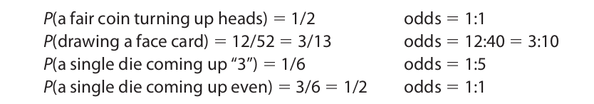
Strictly speaking, of course, the two assumptions underlying the classical theory are never perfectly reflected in any actual situation. Every coin is slightly off balance, as is every pair of dice. As a result, the probabilities of the various outcomes are never exactly equal. Similarly, the outcomes are never strictly confined to the normal ones entailed by the first assumption. When tossing a coin, there is always the possibility that the coin will land on edge, and in rolling dice there is the analogous possibility that one of them might break in half. These outcomes may not be possible in the practical sense, but they are logically possible in that they do not involve any contradiction. Because these outcomes are so unusual, however, it is reasonable to think that for all practical purposes the two assumptions hold and that therefore the classical theory is applicable.

There are many events, however, for which the two assumptions required by the classical theory obviously do not hold. For example, in attempting to determine the probability of a sixty-year-old woman dying of a heart attack within ten years, it would be virtually impossible to take account of all the possible outcomes. She might die of cancer, pneumonia, or an especially virulent case of the flu. She might be incapacitated by a car accident, or she might move to Florida and buy a house on the beach. Furthermore, none of these outcomes is equally probable in comparison with the others. To compute the probability of events such as these we need the relative frequency theory.

The relative frequency theory of probability originated with the use of mortality tables by life insurance companies in the eighteenth century. In contrast with the classical theory, which rests upon a priori computations, the relative frequency theory depends on actual observations of the frequency with which certain events happen. The probability of an event A is given by the formula

where fo is the number of observed favorable outcomes and no is the total number of observed outcomes. For example, to determine the probability that a fifty-year-old man will live five more years, a sample of 1,000 fifty-year-old men could be observed. If 968 were alive five years later, the probability that a fifty-year-old man will live an additional five years is 968/1000 or .968.

Similarly, if one wanted to determine the probability that a certain irregularly shaped pyramid with different colored sides would, when rolled, come to rest with the green side down, the pyramid could be rolled 1,000 times. If it came to rest with its green side down 327 times, the probability of this event happening would be computed to be .327.

The relative frequency method can also be used to compute the probability of the kinds of events that conform to the requirements of the classical theory. For example, the probability of a coin coming up heads could be determined by tossing the coin 100 times and counting the heads. If, after this many tosses, 46 heads have been recorded, one might assign a probability of .46 to this event. This leads us to an important point about the relative frequency theory: The results hold true only in the long run. It might be necessary to toss the coin 1,000 or even 10,000 times to get a close approximation. After 10,000 tosses one would expect to count close to 5,000 heads. If in fact only 4,623 heads have been recorded, one would probably be justified in concluding that the coin is off balance or that something was irregular in the way it had been tossed.

Strictly speaking, neither the classical method nor the relative frequency method can assign a probability to individual events. From the standpoint of these approaches only certain kinds or classes of events have probabilities. But many events in the actual world are unique—for example, Margaret’s marrying Peter or Native Prancer’s winning the fourth race at Churchill Downs. To interpret the probability of these events we turn to the subjectivist theory.

The subjectivist theory of probability interprets the meaning of probability in terms of the beliefs of individual people. Although such beliefs are vague and nebulous, they may be given quantitative interpretation through the odds that a person would accept on a bet. For example, if a person believes that a certain horse will win a race and he or she is willing to give 7 to 4 odds on that event happening, this means that he or she has assigned a probability of 7/(7+4) or 7/11 to that event. This procedure is unproblematic as long as the person is consistent in giving odds on the same event not happening. If, for example, 7 to 4 odds are given that an event will happen and 5 to 4 odds that it will not happen, the individual who gives these odds will inevitably lose. If 7 to 4 odds are given that an event will happen, no better than 4 to 7 odds can be given that the same event will not happen.

One of the difficulties surrounding the subjectivist theory is that one and the same event can be said to have different probabilities, depending on the willingness of different people to give different odds. If probabilities are taken to be genuine attributes of events, this would seem to be a serious problem. The problem might be avoided, though, either by interpreting probabilities as attributes of beliefs or by taking the average of the various individual probabilities as the probability of the event.

11.2 The Probability Calculus

The three theories discussed thus far—the classical theory, the relative frequency theory, and the subjectivist theory—provide separate procedures for assigning a probability to an event (or class of events). Sometimes one theory is more readily applicable, sometimes another. But once individual events have been given a probability, the groundwork has been laid for computing the probabilities of compound arrangements of events. This is done by means of what is called the probability calculus. In this respect the probability calculus functions analogously to the set of truth-functional rules in propositional logic. Just as the truth-functional rules allow us to compute the truth values of compound propositions from the individual truth values of the simple components, the rules of the probability calculus allow us to compute the probability of compound events from the individual probabilities of the simple events.

Two preliminary rules of the probability calculus are (1) the probability of an event that must necessarily happen is taken to be 1, and (2) the probability of an event that necessarily cannot happen is taken to be 0. For example, the event consisting of it either raining or not raining (at the same time and place) has a probability of 1, and the event consisting of it both raining and not raining (at the same time and place) has a probability of 0. These events correspond to statements that are tautological and selfcontradictory, respectively. Contingent events, on the other hand, have probabilities greater than 0 but less than 1. For example, the probability that the Dow Jones Industrial Average will end a certain week at least five points higher than the previous week would usually be around 1/2, the probability that the polar ice cap will melt next year is very close to 0, and the probability that a traffic accident will occur somewhere tomorrow is very close to 1. Let us now consider six additional rules of the probability calculus.

 

1. Restricted Conjunction Rule

The restricted conjunction rule is used to compute the probability of two events occurring together when the events are independent of each other. Two events are said to be independent when the occurrence of one has no effect on the probability of the other one occurring. Examples include getting two heads from two tosses of a coin, drawing two hearts from a deck when the first is replaced before the second is drawn, and playing two sequential games of poker or roulette. The probability of two such events A and B occurring together is given by the formula

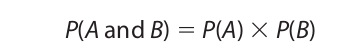
For example, the probability of tossing two heads on a single throw of two coins is

This result may be checked very easily by listing all the possible outcomes and comparing that number with the number of favorable outcomes:

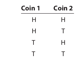
Only one of the four possible outcomes shows both coins turning up heads.

Similarly, we may compute the probability of rolling two sixes with a pair of dice:

Since only one of the thirty-six possible outcomes shows two sixes together, the probability of this event is 1/36.

 

2. General Conjunction Rule

The general conjunction rule is used to compute the probability of two events occurring together whether or not the events are independent. When the events are independent, the general conjunction rule reduces to the restricted conjunction rule. Some examples of events that are not independent (that is, that are dependent) are drawing two spades from a deck on two draws when the first card drawn is not replaced, and selecting two or more window seats on an airplane. After the first card is drawn, the number of cards available for the second draw is reduced, and after one of the seats is taken on the plane, the number of seats remaining for subsequent choices is reduced. In other words, in both cases the second event is dependent on the first. The formula for computing the probability of two such events occurring together is

The expression P(B given A) is the probability that B will occur on the assumption that A has already occurred. Let us suppose, for example, that A and B designate the events of drawing two kings from a deck when the first card is not replaced before the second is drawn. If event A occurs, then only three kings remain, and the deck is also reduced to fifty-one cards. Thus, P(B given A) is 3/51. Since the probability of event A is 4/52, the probability of both events happening is the product of these two fractions, or 12/2652 (= 1/221).

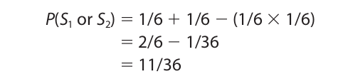
For another illustration, consider an urn containing five red balls, six green balls, and seven yellow balls. The probability of drawing two red balls (without replacement) is computed as follows:

If a red ball is selected on the first draw, this leaves four red balls from a total of seventeen. Thus, the probability of drawing a second red ball if one has already been drawn is 4/17.

For another example, consider the same urn with the same contents, but let us compute the probability of drawing first a green ball and then a yellow ball (without replacement):

If a green ball is selected on the first draw, this affects the selection of a yellow ball on the second draw only to the extent of reducing the total number of balls to seventeen.

 

3. Restricted Disjunction Rule

The restricted disjunction rule is used to compute the probability of either of two events occurring when the events are mutually exclusive—that is, when they cannot both occur. Examples of such events include picking either an ace or a king from a deck of cards on a single draw or rolling either a six or a one on a single roll of a die. The probability is given by the formula

For example, the probability of drawing either a king or a queen (of any suit) from a deck of cards on a single draw is

For another example, consider an urn containing six black balls, four white balls, and two red balls. The probability of selecting either a black or red ball on a single draw is

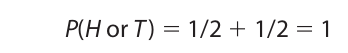
When the event in question is one that must necessarily occur, the probability is, of course, 1. Thus, the probability of obtaining either heads or tails on a single toss of a coin is

The restricted disjunction rule may be combined with the restricted conjunction rule to compute the probability of getting either a five or a six on each of two consecutive rolls of a single die:

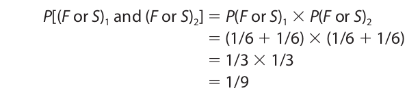
Since getting a five and getting a six on a single die are mutually exclusive events, P(F or S) 1 is evaluated using the restricted disjunction rule. The same is true of P(F or S)2. Then, since two rolls of a die are independent events, the conjunction of the two disjunctive events is evaluated by the restricted conjunction rule.

 

4. General Disjunction Rule

The general disjunction rule is used to compute the probability of either of two events whether or not they are mutually exclusive. The rule holds for any two events, but since its application is simplified when the events are independent, we will confine our attention to events of this kind. Examples of independent events that are not mutually exclusive include obtaining at least one head on two tosses of a coin, drawing at least one king from a deck on two draws when the first card is replaced before the second card is drawn, and getting at least one six when rolling a pair of dice. The formula for computing the probability of either of two such events is

If the events are independent, P(A and B) is computed using the restricted conjunction rule, and the general disjunction formula reduces to

The general disjunction rule may be proved as follows. When A and B are nonexclusive, A occurs either with or without B, and B occurs either with or without A. Thus,

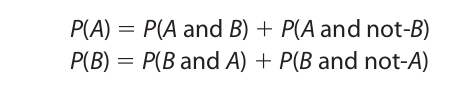
But A or B occurs in exactly three possible ways: A and not-B, B and not-A, and A and B. Thus,

Thus, when P(A and B) is subtracted from P(A) + P(B), the difference is equal to P(A or B). [Note: P(A and B) = P(B and A).]

For an example of the use of the general disjunction rule let us consider the probability of getting heads on either of two tosses of a coin. We have

For another example, consider the probability of getting at least one six when rolling a pair of dice. The computation is

The general disjunction rule may be combined with the restricted disjunction rule to compute the probability of getting either a three or a five when rolling a pair of dice. This is the probability of getting either a three or a five on the first die or either a three or a five on the second:

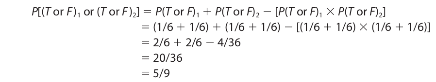
Since getting a three or getting a five on a single throw are mutually exclusive events, P(T or F) 1 is equal to the sum of the separate probabilities. The same is true for P(T or F)2.

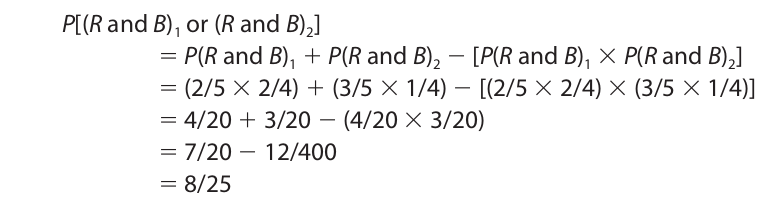
The general disjunction rule may be combined with the general conjunction rule to compute the probability of drawing first a red ball and then a black ball on pairs of draws from either of two urns (without replacement). Suppose that the first urn contains two red balls, two black balls, and one green ball, and that the second urn contains three red balls, one black ball, and one white ball. The probability, giving two draws per urn, is

 

 

5. Negation Rule

The negation rule is useful for computing the probability of an event when the probability of the event not happening is either known or easily computed. The formula is as follows:

The formula can be proved very easily. By the restricted disjunction rule the probability of A or not-A is

But since A or not-A happens necessarily, P(A or not-A) = 1. Thus,

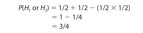
Rearranging the terms in this equation gives us the negation rule. For an example of the use of this rule, consider the probability of getting heads at least once on two tosses of a coin. The probability of the event not happening, which is the probability of getting tails on both tosses, is immediately computed by the restricted conjunction rule to be 1/4. Then, applying the negation rule, we have

The negation rule may also be used to compute the probabilities of disjunctive events that are dependent. In presenting the general disjunction rule we confined our attention to independent events. Let us suppose we are given an urn containing two black balls and three white balls. To compute the probability of getting at least one black ball on two draws (without replacement), we first compute the probability of the event not happening. This event consists in drawing two white balls, which, by the general conjunction rule, has the probability

Now, applying the negation rule, the probability of getting at least one black ball on two draws is

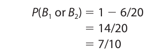
For an example that is only slightly more complex, consider an urn containing two white, two black, and two red balls. To compute the probability of getting either a white or black ball on two draws (without replacement) we first compute the probability of the event not happening. This is the probability of getting red balls on both draws, which is

Now, by the negation rule the probability of drawing either a white or black ball is

 

6. Bayes’s Theorem

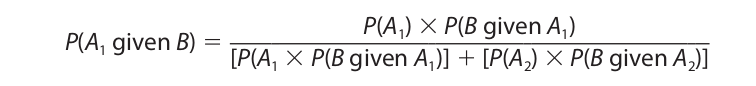
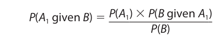
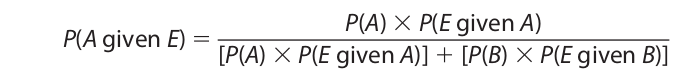
Bayes’s theorem, named after the eighteenth-century English clergyman Thomas Bayes, is a useful rule for evaluating the conditional probability of two or more mutually exclusive and jointly exhaustive events. The conditional probability of an event is the probability of that event happening given that another event has already happened, and it is expressed P(A given B). You may recall that an expression of this form occurred in the formulation of the general conjunction rule. When the number of mutually exclusive and jointly exhaustive events is limited to two, which we will designate A1 and A2, Bayes’s theorem is expressed as follows:

This limited formulation of Bayes’s theorem may be proved as follows. Applying the general conjunction rule to the events A1 and B, we have

Applying the same rule to the same events written in the reverse order, we have

Now, since P(A1 and B) is equal to P(B and A1), we may set the right-hand side of these two equations equal to each other:

Dividing both sides of this equation by P(B), we have

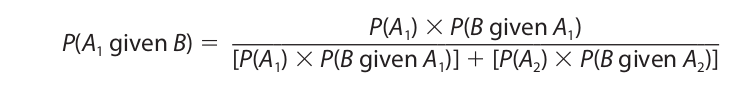
Now, it can be easily proved using a truth table that B is logically equivalent to the expression [(A1 and B) or (not-A1 and B)]. Furthermore, since A1 and A2 are mutually exclusive and jointly exhaustive, one and only one of them will happen. Thus, A2 is simply another way of writing not-A1. Accordingly, the former expression in brackets can be written [(A1 and B) or (A2 and B)], and since this expression is logically equivalent to B,

Now, applying the general conjunction rule and the restricted disjunction rule to the right-hand side of this equation, we have

Finally, substituting the right-hand side of this equation in place of P(B) in the earlier equation marked (*), we have Bayes’s theorem:

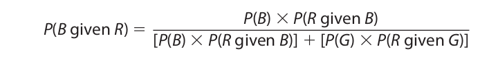
For an illustration of the use of Bayes’s theorem, suppose we are given one beige urn and four gray urns in a dimly lit room, so we cannot distinguish one color from the other. The beige urn contains eight red and two white balls, and each of the gray urns contains three red and seven white balls. Suppose that a red ball is drawn from one of these five urns. What is the probability that the urn was beige? In other words, we want to know the probability that the urn was beige given that a red ball was drawn. The events A1 and A2 in Bayes’s theorem correspond to drawing a ball from either a beige urn or a gray urn. Substituting B and G for A1 and A2, respectively, we have

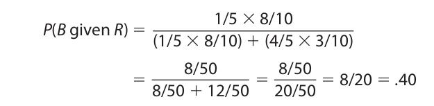
Now, since there are a total of five urns, the probability of randomly selecting the beige urn is 1/5, and the probability of randomly selecting one of the gray urns is 4/5. Finally, since each urn contains ten balls, the probability of drawing a red ball from the beige urn is 8/10, and the probability of drawing a red ball from the gray urn is 3/10. Thus, we have

Bayes’s theorem is quite practical because it allows us to change our probability estimates of ordinary events as new information is acquired. For an example of how Bayes’s theorem is used for this purpose, consider the following example:

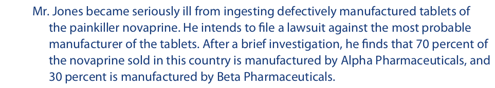
From this information the probability that Alpha Pharmaceuticals manufactured the tablets is .70, in comparison with .30 for Beta Pharmaceuticals. Thus, Mr. Jones tentatively decides to file his lawsuit against Alpha. However, on further investigation Mr. Jones discovers the following:

Clearly this new information affects Mr. Jones’s original probability estimate. We use Bayes’s Theorem to recompute the probability that Alpha manufactured the defective tablets given that the tablets were purchased on the East Coast as follows:

For P(A) and P(B) we use the original probabilities of .70 and .30, respectively. The probability that the tablets were purchased on the East Coast given that they were manufactured by Alpha is .10, and the probability that they were purchased on the East Coast given that they were manufactured by Beta is .80. Thus, we have

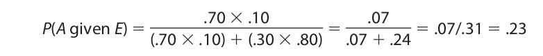
The new information that Mr. Jones acquired has significantly affected the probability that Alpha manufactured the defective tablets. The probability has dropped from .70 to .23. With this new information, it is more likely that Beta manufactured the tablets, so Mr. Jones should now file his lawsuit against Beta. The probability for Beta is 1 − .23, or .77.

The earlier probability for Alpha (.70) is called the prior probability, and the later figure (.23) is called the posterior probability. If Mr. Jones should acquire even more information, the posterior probability becomes a new prior, and it is used as the value for P(A) in a subsequent application of Bayes’s theorem.

 

Additional Applications

Most of the examples considered thus far have used the classical theory to determine the probability of the component events. But as was mentioned earlier, the probability calculus can also be used in conjunction with the relative frequency theory and the subjectivist theory. If we apply the relative frequency theory to the mortality tables used by insurance companies, we find that the probability of a twenty-five-year-old man living an additional forty years is .82, and the probability of a twenty-five-yearold woman living the same number of years is .88. To compute the probability of such a man and woman both living that long, we use the restricted conjunction rule and obtain .82 × .88 = .72. For the probability that either of these people would live that long, we use the general disjunction rule and obtain

Let us suppose that these two people are married and both would give 9 to 1 odds on their staying married for forty years. This translates into a probability of 9/(9 + 1) or .90. Using the restricted conjunction rule, the probability of this event happening is the product of the latter figure and the probability of their both living that long, or .65.

For an example involving the subjectivist theory, if the Philadelphia Eagles are given 7 to 5 odds of winning the NFC championship, and the New England Patriots are given 3 to 2 odds of winning the AFC championship, the probability that at least one of these teams will win is computed using the general disjunction rule. The odds translate respectively into probabilities of 7/12 and 3/5, and so the probability of the disjunction is 7/12 + 3/5 − (7/12 × 3/5) = 5/6. The probability that the two teams will meet in the Super Bowl (that both will win their conference championship) is, by the restricted conjunction rule, 7/12 × 3/5 = 21/60, or 7/20. The probability that neither will play in the Super Bowl is, by the negation rule, 1 − 5/6 = 1/6.

The probability calculus can also be used to evaluate the strength of inductive arguments. Consider the following:

On the assumption that the premises are true, that is, on the assumption that the odds are reported correctly, the conclusion follows with a probability of 7/20 or .35. Thus, the argument is not particularly strong. But if the odds given in the premises should increase, the strength of the argument would increase proportionately. The premises of the following argument give different odds:

In this argument, if the premises are assumed true, the conclusion follows with a probability of 7/9 × 8/11 = 56/99, or .57. Thus, the argument is at least moderately strong.

Lest this procedure be misinterpreted, however, we should recall a point raised in Chapter 1. The strength of an inductive argument depends not merely on whether the conclusion is probably true but on whether the conclusion follows probably from the premises. As a result, to evaluate the strength of an inductive argument it is not sufficient merely to know the probability of the conclusion on the assumption that the premises are true. One must also know whether the probability of the conclusion rests on the evidence given in the premises. If the probability of the conclusion does not rest on this evidence, the argument is weak regardless of whether the conclusion is probably true. The following argument is a case in point:

The conclusion of this argument is probably true independently of the premises, so the argument is weak.

In this connection the analogy between deductive and inductive arguments breaks down. As we saw in Chapter 6, any argument having a conclusion that is necessarily true is deductively valid regardless of the content of its premises. But any inductive argument having a probably true conclusion is not strong unless the probability of the conclusion rests on the evidence given in the premises.

A final comment is in order about the material covered in this chapter. Probability is one of those subjects about which there is little agreement among philosophers. Some philosophers defend each of the theories we have discussed as providing the only acceptable approach, and there are numerous views regarding the fine points of each. However, some philosophers argue that there are certain uses of “probability” that none of these theories can interpret. The statement “There is high probability that Einstein’s theory of relativity is correct” may be a case in point. In any event, the various theories about the meaning of probability, as well as the details of the probability calculus, are highly complex subjects, and the brief account given here has merely scratched the surface.

 

Chapter 12: Statistical Reasoning

12.1 Evaluating Statistics

In our day-to-day experience all of us encounter arguments that rest on statistical evidence. An especially prolific source of such arguments is the advertising industry. We are constantly told that we ought to sign up with a certain cell phone service because it has 30 percent fewer dropped calls, buy a certain kind of car because it gets 5 percent better gas mileage, and use a certain cold remedy because it is recommended by four out of five physicians. But the advertising industry is not the only source. We often read in the newspapers that some union is asking an increase in pay because its members earn less than the average or that a certain region is threatened with floods because rainfall has been more than the average.

To evaluate such arguments, we must be able to interpret the statistics on which they rest, but doing so is not always easy. Statements expressing averages and percentages are often ambiguous and can mean a variety of things, depending on how the average or percentage is computed. These difficulties are compounded by the fact that statistics provide a highly convenient way for people to deceive one another. Such deceptions can be effective even though they fall short of being outright lies. Thus, to evaluate arguments based on statistics one must be familiar not only with the ambiguities that occur in the language but with the devices that unscrupulous individuals use to deceive others.

This chapter touches on five areas that are frequent sources of such ambiguity and deception: problems in sampling, the meaning of “average,” the importance of dispersion in a sample, the use of graphs and pictograms, and the use of percentages for the purpose of comparison. By becoming acquainted with these topics and with some of the misuses that occur, we improve our ability to determine whether a conclusion follows probably from a set of statistical premises.

12.2 Samples

Much of the statistical evidence presented in support of inductively drawn conclusions is gathered from analyzing samples. When a sample is found to possess a certain characteristic, it is argued that the group as a whole (the population) possesses that characteristic. For example, if we wanted to know the opinion of the student body at a certain university about whether to adopt an academic honor code, we could take a poll of 10 percent of the students. If the results of the poll showed that 80 percent of those sampled favored the code, we might draw the conclusion that 80 percent of the entire student body favored it. Such an argument would be classified as an inductive generalization.

The problem that arises with the use of samples has to do with whether the sample is representative of the population. Samples that are not representative are said to be biased samples. Depending on what the population consists of, whether machine parts or human beings, different considerations enter into determining whether a sample is biased. These considerations include (1) whether the sample is randomly selected, (2) the size of the sample, and (3) psychological factors.

A random sample is one in which every member of the population has an equal chance of being selected. The requirement that a sample be randomly selected applies to practically all samples, but sometimes it can be taken for granted. For example, when a physician draws a blood sample to test for blood sugar, there is no need to take a little bit from the finger, a little from the arm, and a little from the leg. Because blood is a circulating fluid, it can be assumed that it is homogenous in regard to blood sugar.

The randomness requirement demands more attention when the population consists of discrete units. Suppose, for example, that a quality-control engineer for a manufacturing firm needed to determine whether the components on a certain conveyor belt were within specifications. To do so, the engineer removed every tenth component for measurement. The sample obtained by such a procedure would not be random if the components were not randomly arranged on the conveyor belt. As a result of some malfunction in the manufacturing process it is quite possible that every tenth component was perfect and the rest were imperfect. If the engineer happened to select only the perfect ones, the sample would be biased. A selection procedure that would be more likely to ensure a random sample would be to roll a pair of dice and remove every component corresponding to a roll of ten. Since the outcome of a roll of dice is a random event, the selection would also be random. Such a procedure would be more likely to include defective components that turn up at regular intervals.

The randomness requirement presents even greater problems when the population consists of human beings. Suppose, for example, that a public opinion poll is to be conducted on the question of excessive corporate profits. It would hardly do to ask such a question randomly of the people encountered on Wall Street in New York City. Such a sample would almost certainly be biased in favor of the corporations. A less biased sample could be obtained by randomly selecting phone numbers from the telephone directory, but even this procedure would not yield a completely random sample. Among other things, the time of day in which a call is placed influences the kind of responses obtained. Most people who are employed full-time are not available during the day, and even if calls are made at night, a large percentage of the population have unlisted numbers.

A poll conducted by mail based on the addresses listed in the city directory would also yield a fairly random sample, but this method, too, has shortcomings. Many apartment dwellers are not listed, and others move before the directory is printed. Furthermore, none of those who live in rural areas are listed. In short, it is both difficult and expensive to conduct a large-scale public opinion poll that succeeds in obtaining responses from anything approximating a random sample of individuals.

A classic case of a poll that turned out to be biased in spite of a good deal of effort and expense occurred when the Literary Digest magazine undertook a poll to predict the outcome of the 1936 presidential election. The sample consisted of a large number of the magazine’s subscribers together with other people selected from the telephone directory. Because four similar polls had picked the winner in previous years, the results of this poll were highly respected. As it turned out, however, the Republican candidate, Alf Landon, got a significant majority in the poll, but Franklin D. Roosevelt won the election by a landslide. The incorrect prediction is explained by the fact that the 1936 election occurred in the middle of the Depression, at a time when many people could afford neither a telephone nor a subscription to the Digest. These were the people who were overlooked in the poll, and they were also the ones who voted for Roosevelt.

Size is also an important factor in determining whether a sample is representative. Given that a sample is randomly selected, the larger the sample, the more closely it replicates the population. In statistics, this degree of closeness is expressed in terms of sampling error. The sampling error is the difference between the relative frequency with which some characteristic occurs in the sample and the relative frequency with which the same characteristic occurs in the population. If, for example, a poll were taken of a labor union and 60 percent of the members sampled expressed their intention to vote for Smith for president but in fact only 55 percent of the whole union intended to vote for Smith, the sampling error would be 5 percent. If a larger sample were taken, the error would be smaller.

Just how large a sample should be is a function of the size of the population and of the degree of sampling error that can be tolerated. For a sampling error of, say, 5 percent, a population of 10,000 would require a larger sample than would a population of 100. However, the ratio is not linear. To obtain the same precision, the sample for the larger population need not be 100 times as large as the one for the smaller population. When the population is very large, the size of the sample needed to ensure a certain precision levels off at a constant figure. For example, a random sample of 500 will yield results that are just as accurate whether the population is 100 thousand or 100 million.

When the population is very large, and the sample is random and less than 5 percent of the population, sampling error can be expressed in terms of a mathematical margin of error as per Table 12.1:

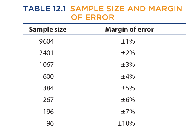
The figures in this table are based on a 95% level of confidence, which means that we can be 95% certain that a sample will accurately reflect the whole population within the margin of error for that sample. Thus, if from a random poll of 9604 people, 53 percent say they prefer Jones for governor, then we can be 95 percent certain that between 52 and 54 percent of the whole population prefers Jones. The figures in the table are based purely on mathematics and are not dependent on any empirical measurement. For a 95 percent confidence level, the margin of error is approximately equal to .98/√n, where n is the size of the sample. For a 99 percent confidence level, the margin of error is approximately equal to 1.29/√n. Comparing these two expressions shows that as the confidence level increases, so does the margin of error.

In most polls, the margin of error is based on a 95 percent (or higher) confidence level. But if a much lower confidence level should be selected, and if this fact is not disclosed, then the results of a poll could be deceptive—even if the margin of error is stated. The reason for this is that the margin of error would be combined with a low likelihood that it covered any actual discrepancy between the sample and the population. Also, of course, any poll that simply fails to disclose the margin of error can be deceptive. For example, if a poll should show Adams leading Baker for U.S. Senate by 55 to 45 percent, this means virtually nothing if neither the size of the sample nor the margin of error is given. If the margin of error should be as high as 10 percent, then it could be the case that it is Baker who leads Adams by 55 to 45 percent.

Even when the margin of error is stated, however, incorrect conclusions are often drawn when comparing the results of one poll with the results of another. Suppose a poll shows Adams leading Baker by 55 to 45 percent. After an article critical of Adams appears in the newspaper, a second poll is taken that shows Adams trailing Baker by 49 to 51 percent. Suppose further that the margin of error for both polls is 4 percent and the confidence level is 95 percent. From such polls people often draw the conclusion that Adam’s lead over Baker has disappeared, when in fact no such conclusion is warranted. Taking into account the margin of error, it could be the case that in fact Adams’s lead over Baker has remained constant at, say, 53 to 47 percent.

Statements of sampling error are often conspicuously absent from surveys used to support advertising claims. Marketers of products such as patent medicines have been known to take rather small samples until they obtain one that gives the “right” result. For example, twenty polls of twenty-five people might be taken inquiring about the preferred brand of aspirin. Even though the samples might be randomly selected, one will eventually be found in which twenty of the twenty-five respondents indicate their preference for Alpha brand aspirin. Having found such a sample, the marketing firm proceeds to promote this brand as the one preferred by four out of five of those sampled. The results of the other samples are, of course, discarded, and no mention is made of sampling error.

Psychological factors can also have a bearing on whether the sample is representative. When the population consists of inanimate objects, such as cans of soup or machine parts, psychological factors are usually irrelevant, but they can play a significant role when the population consists of human beings. If the people composing the sample think that they will gain or lose something by the kind of answer they give, their involvement will likely affect the outcome. For example, if the residents of a neighborhood were to be surveyed for annual income with the purpose of determining whether the neighborhood should be ranked among the fashionable areas in the city, we would expect the residents to exaggerate their answers. But if the purpose of the study were to determine whether the neighborhood could afford a special levy that would increase property taxes, we might expect the incomes to be underestimated.

The kind of question asked can also have a psychological bearing. Questions such as “How often do you brush your teeth?” and “How many books do you read in a year?” can be expected to generate responses that overestimate the truth, while “How many times have you been intoxicated?” and “How many extramarital affairs have you had?” would probably receive answers that underestimate the truth. Similar exaggerations can result from the way a question is phrased. For example, “Do you favor a reduction in welfare benefits as a response to rampant cheating?” would be expected to receive more affirmative answers than simply “Do you favor a reduction in welfare benefits?”

Another source of psychological influence is the personal interaction between the surveyor and the respondent. Suppose, for example, that a door-to-door survey were taken to determine how many people believe in God or attend church on Sunday. If the survey were conducted by priests and ministers dressed in clerical garb, one might expect a larger number of affirmative answers than if the survey were taken by nonclerics. The simple fact is that many people like to give answers that please the questioner.

To prevent this kind of interaction from affecting the outcome, scientific studies are often conducted under “double blind” conditions in which neither the surveyor nor the respondent knows what the “right” answer is. For example, in a double blind study to determine the effectiveness of a drug, bottles containing the drug would be mixed with other bottles containing a placebo (sugar tablet). The contents of each bottle would be matched with a code number on the label, and neither the person distributing the bottles nor the person recording the responses would know what the code is. Under these conditions the people conducting the study would not be able to influence, by some smile or gesture, the response of the people to whom the drugs are given.

Most of the statistical evidence encountered in ordinary experience contains no reference to such factors as randomness, sampling error, or the conditions under which the sample was taken. In the absence of such information, the person faced with evaluating the evidence must use his or her best judgment. If either the organization conducting the study or the people composing the sample have something to gain by the kind of answer that is given, the results of the survey should be regarded as suspect. And if the questions that are asked concern topics that would naturally elicit distorted answers, the results should probably be rejected. In either event, the mere fact that a study appears scientific or is expressed in mathematical language should never intimidate a person into accepting the results. Numbers and scientific terminology are no substitute for an unbiased sample.

 

12.3 The Meaning of “Average”

In statistics the word “average” is used in three different senses: mean, median, and mode. In evaluating arguments and inferences that rest on averages, we often need to know in precisely what sense the word is being used.

The mean value of a set of data is the arithmetical average. It is computed by dividing the sum of the individual values by the number of values in the set. Suppose, for example, that we are given Table 12.2 listing the ages of a group of people. To compute the mean age, we divide the sum of the individual ages by the number of people:

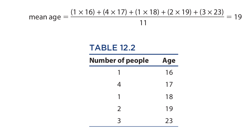
The median of a set of data is the middle point when the data are arranged in ascending order. In other words, the median is the point at which there is an equal number of data above and below. In Table 12.2 the median age is 18 because there are five people above this age and five below.

The mode is the value that occurs with the greatest frequency. Here the mode is 17, because there are four people with that age and fewer people with any other age.

In this example, the mean, median, and mode differ but are all fairly close together. The problem for induction occurs when a great disparity among these values occurs. This sometimes occurs in the case of salaries. Consider, for example, Table 12.3, which reports the salaries of a hypothetical architectural firm. Since there are twenty-one employees and a total of $1,365,000 is paid in salaries, the mean salary is $1,365,000/21, or $65,000. The median salary is $45,000 because ten employees earn less than this and ten earn more, and the mode, which is the salary that occurs most frequently, is $30,000. Each of these figures represents the “average” salary of the firm, but in different senses. Depending on the purpose for which the average is used, different figures might be cited as the basis for an argument.

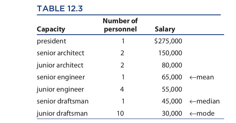
For example, if the senior engineer were to request a raise in salary, the president could respond that his or her salary is already well above the average (in the sense of median and mode) and that therefore that person does not deserve a raise. If the junior draftsmen were to make the same request, the president could respond that they are presently earning the firm’s average salary (in the sense of mode), and that for draftsmen to be earning the average salary is excellent. Finally, if someone from outside the firm were to allege that the firm pays subsistence-level wages, the president could respond that the average salary of the firm is a hefty $65,000. All of the president’s responses would be true, but if the reader or listener were not sophisticated enough to distinguish the various senses of “average,” he or she might be persuaded by the arguments.

In some situations, the mode is the most useful average. Suppose, for example, that you are in the market for a three-bedroom house. Suppose further that a real estate agent assures you that the houses in a certain complex have an average of three bedrooms and that therefore you will certainly want to see them. If the agent has used “average” in the sense of mean, it is possible that half the houses in the complex are four-bedroom, the other half are two-bedroom, and there are no three-bedroom houses at all. A similar result is possible if the agent has used average in the sense of median. The only sense of average that would be useful for your purposes is mode: If the modal average is three bedrooms, there are more three-bedroom houses than any other kind.

On other occasions a mean average is the most useful. Suppose, for example, that you have taken a job as a pilot on a plane that has nine passenger seats and a maximum carrying capacity of 1,350 pounds (in addition to yourself). Suppose further that you have arranged to fly a group of nine passengers over the Grand Canyon and that you must determine whether their combined weight is within the required limit. If a representative of the group tells you that the average weight of the passengers is 150 pounds, this by itself tells you nothing. If he means average in the sense of median, it could be the case that the four heavier passengers weigh 200 pounds and the four lighter ones weigh 145, for a combined weight of 1,530 pounds. Similarly, if the passenger representative means average in the sense of mode, it could be that two passengers weigh 150 pounds and that the others have varying weights in excess of 200 pounds, for a combined weight of over 1,700 pounds. Only if the representative means average in the sense of mean do you know that the combined weight of the passengers is 9 × 150 or 1,350 pounds.

Finally, sometimes a median average is the most meaningful. Suppose, for example, that you are a manufacturer of a product that appeals to people under age thirty-five. To increase sales you decide to run an ad in a national magazine, but you want some assurance that the ad will be read by the right age group. If the advertising director of a magazine tells you that the average age of the magazine’s readers is 35, you know virtually nothing. If the director means average in the sense of mean, it could be that 90 percent of the readers are over 35 and that the remaining 10 percent bring the average down to 35. Similarly, if the director means average in the sense of mode, it could be that 3 percent of the readers are exactly 35 and that the remaining 97 percent have ages ranging from 35 to 85. Only if the director means average in the sense of median do you know that half the readers are 35 or less.

 

12.4 Dispersion

Although averages often yield important information about a set of data, there are many cases in which merely knowing the average, in any sense of the term, tells us very little. The reason for this is that the average says nothing about how the data are distributed. For this, we need to know something about dispersion, which refers to how spread out the data are in regard to numerical value. Three important measures of dispersion are range, variance, and standard deviation.

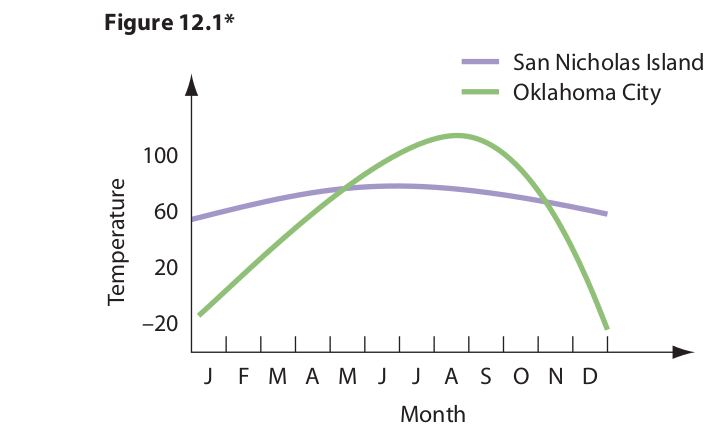
Let us first consider the range of a set of data, which is the difference between the largest and the smallest values. For an example of the importance of this parameter, suppose that after living for many years in an intemperate climate, you decide to relocate in an area that has a more ideal mean temperature. On discovering that the annual mean temperature of Oklahoma City is 60°F you decide to move there, only to find that you roast in the summer and freeze in the winter. Unfortunately, you had ignored the fact that Oklahoma City has a temperature range of 130°, extending from a record low of −17° to a record high of 113°. In contrast, San Nicholas Island, off the coast of California, has a mean temperature of 61° but a range of only 40°, extending from 47° in the winter to 87° in the summer. The temperature ranges for these two locations are approximated in Figure 12.1.

Even granting the importance of the range of the data in this example, however, range really tells us relatively little because it comprehends only two data points, the maximum and minimum. It says nothing about how the other data points are distributed. For this we need to know the variance, or the standard deviation, which measure how every data point varies or deviates from the mean.

For an example of the importance of these two parameters in describing a set of data, suppose you have a four-year-old child and you are looking for a day-care center that will provide plenty of possible playmates about the same age as your child. After calling several centers on the phone, you narrow the search down to two: the Rumpus Center and the Bumpus Center. Both report that they regularly care for nine children, that the mean and median age of the children is four, and that the range in ages of the children is six. Unable to decide between these two centers, you decide to pay them a visit. Having done so, you see that the Rumpus Center will meet your needs better than the Bumpus Center. The reason is that the ages of the children in the two centers are distributed differently.

The ages of the children in the two centers are as follows:

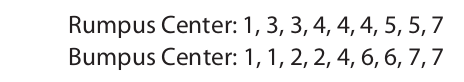
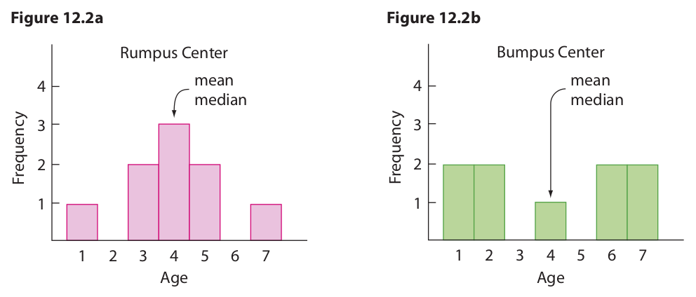
To illustrate the differences in distribution, these ages can be plotted on a certain kind of bar graph, called a histogram, as shown in Figures 12.2a and 12.2b. Obviously the reason why the Rumpus Center comes closer to meeting your needs is that it has seven children within one year of your own child, whereas the Bumpus Center has only one such child. This difference in distribution is measured by the variance and the standard deviation. Computing the value of these parameters for the two centers is quite easy, but first we must introduce some symbols. The standard deviation is represented in statistics by the Greek letter σ (sigma), and the variance, which is the square of the standard deviation, is represented by σ2. We compute the variance first, which is defined as follows:

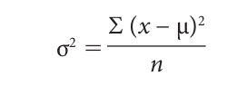
In this expression (which looks far more complicated than it is), ∑ (uppercase sigma) means “the sum of,” x is a variable that ranges over the ages of the children, the Greek letter μ (mu) is the mean age, and n is the number of children. Thus, to compute the variance, we take each of the ages of the children, subtract the mean age (4) from each, square the result of each, add up the squares, and then divide the sum by the number of children (9). The first three steps of this procedure for the Rumpus Center are reported in Table 12.4.

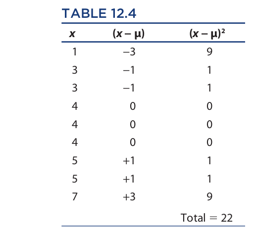
First, the column for x (the children’s ages) is entered, next the column for (x − μ), and last the column for (x − μ)2. After adding up the figures in the final column, we obtain the variance by dividing the sum (22) by n (9):

Finally, to obtain the standard deviation, we take the square root of the variance:

Next, we can perform the same operation on the ages of the children in the Bumpus Center. The figures are expressed in Table 12.5.

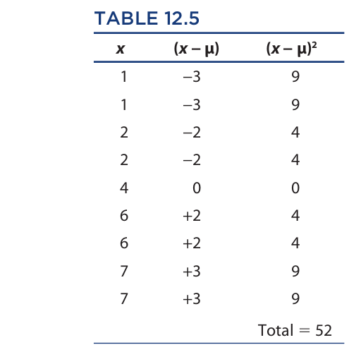
Now, for the variance, we have

And for the standard deviation, we have

These figures for the variance and standard deviation reflect the difference in distribution shown in the two histograms. In the histogram for the Rumpus Center, the ages of most of the children are clumped around the mean age (4). In other words, they vary or deviate relatively slightly from the mean, and this fact is reflected in relatively small figures for the variance (2.44) and the standard deviation (1.56). On the other hand, in the histogram for the Bumpus center, the ages of most of the children vary or deviate relatively greatly from the mean, so the variance (5.78) and the standard deviation (2.40) are larger.

One of the more important kinds of distribution used in statistics is called the normal probability distribution, which expresses the distribution of random phenomena in a population. Such phenomena include (approximately) the heights of adult men or women in a city, the useful life of a certain kind of tire or light bulb, and the daily sales figures of a certain grocery store. To illustrate this concept, suppose that a certain college has 2,000 female students. The heights of these students range from 57 inches to 73 inches. If we divide these heights into one-inch intervals and express them in terms of a histogram, the resulting graph would probably look like the one in Figure 12.3a.

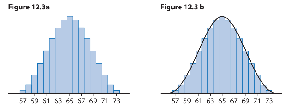
This histogram has the shape of a bell. When a continuous curve is superimposed on top of this histogram, the result appears in Figure 12.3b. This curve is called a normal curve, and it represents a normal distribution. The heights of all of the students fit under the curve, and each vertical slice under the curve represents a certain subset of these heights. The number of heights trails off toward zero at the extreme left and right ends of the curve, and it reaches a maximum in the center. The peak of the curve reflects the average height in the sense of mean, median, and mode.

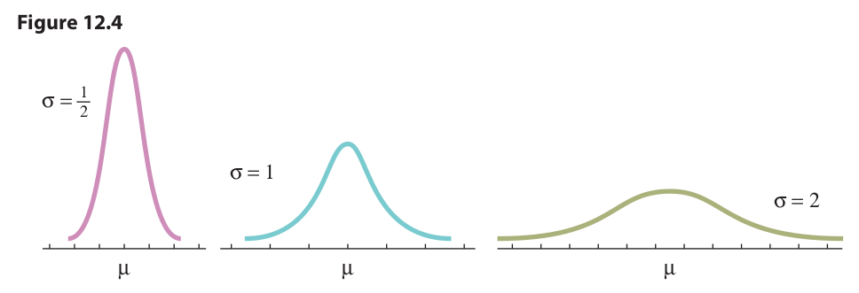
The parameters of variance and standard deviation apply to normal distributions in basically the same way as they do for the histograms relating to the day-care centers. Normal curves with a relatively small standard deviation tend to be relatively narrow and pointy, with most of the population clustered close to the mean, while curves with a relatively large standard deviation tend to be relatively flattened and stretched out, with most of the population distributed some distance from the mean. This idea is expressed in Figure 12.4. As usual, σ represents the standard deviation, and μ represents the mean.

For a final example that illustrates the importance of dispersion, suppose that you decide to put your life savings into a business that designs and manufactures women’s dresses. As corporation president you decide to save money by restricting production to dresses that fit the average woman. Because the average size in the sense of mean, median, and mode is 12, you decide to make only size 12 dresses. Unfortunately, you later discover that while size 12 is indeed the average, 95 percent of women fall outside this interval, as Figure 12.5 shows.

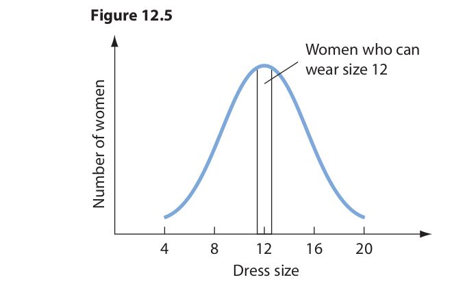
The problem is that you failed to take into account the standard deviation. If the standard deviation were relatively small, then most of the dress sizes would be clustered about the mean (size 12). But in fact the standard deviation is relatively large, so most of the dress sizes fall outside this interval.

 

12.5 Graphs and Pictograms

Graphs provide a highly convenient and informative way to represent statistical data, but they are also susceptible to misuse and misinterpretation. Here we will confine our attention to some of the typical ways in which graphs are misused.

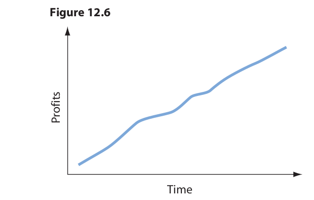
First of all, if a graph is to represent an actual situation, it is essential that both the vertical and horizontal axes be scaled. Suppose, for example, that the profit level of a corporation is represented by a graph such as Figure 12.6. Such a graph is practically meaningless because it fails to show how much the profits increased over what period of time. If the curve represents a 10 percent increase over twenty years, then, of course, the picture is not very bright. Although they convey practically no information, graphs of this kind are used quite often in advertising. A manufacturer of vitamins, for example, might print such a graph on the label of the bottle to suggest that a person’s energy level is supposed to increase dramatically after taking the tablets. Such ads frequently make an impression because they look scientific, and the viewer rarely bothers to check whether the axes are scaled or precisely what the curve is supposed to signify.

A graph that more appropriately represents corporate profits is given in Figure 12.7 (the corporation is fictitious).

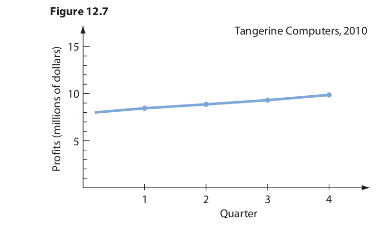
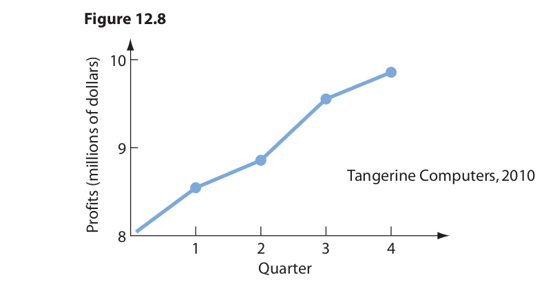
Inspection of the graph reveals that between January and December profits rose from $8 to $10 million, which represents a respectable 25 percent increase. This increase can be made to appear even more impressive by chopping off the bottom of the graph and altering the scale on the vertical axis while leaving the horizontal scale as is (Figure 12.8). Again, strictly speaking, the graph accurately represents the facts, but if the viewer fails to notice what has been done to the vertical scale, he or she is liable to derive the impression that the profits have increased by something like a hundred percent or more.

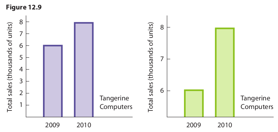
The same strategy can be used with bar graphs. The graphs in Figure 12.9 compare sales volume for two consecutive years, but the one on the right conveys the message more dramatically. Of course, if the sales volume has decreased, the corporate directors would probably want to minimize the difference, in which case the design on the left is preferable.

An even greater illusion can be created with the use of pictograms. A pictogram is a diagram that compares two situations through drawings that differ either in size or in the number of entities depicted. Consider Figure 12.10, which illustrates the increase in production of an oil company between 2005 and 2010.

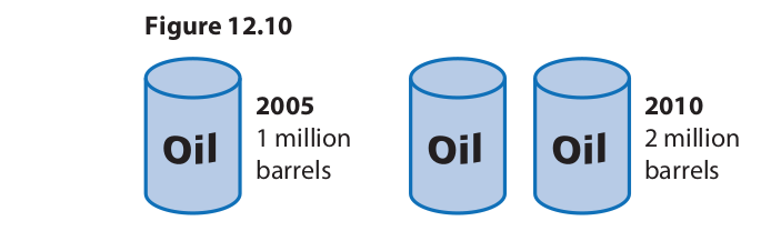
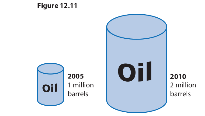
This pictogram accurately represents the increase because it unequivocally shows that the amount doubled between the years represented. But the effect is not especially dramatic. The increase in production can be exaggerated by representing the 2010 level with an oil barrel twice as tall (Figure 12.11).

Even though the actual production is stated adjacent to each drawing, this pictogram creates the illusion that production has much more than doubled. While the drawing on the right is exactly twice as high as the one on the left, it is also twice as wide. Thus, it occupies four times as much room on the page. Furthermore, when the viewer’s threedimensional judgment is called into play, the barrel on the right is perceived as having eight times the volume of the one on the left. Thus, when the third dimension is taken into account, the increase in consumption is exaggerated by 600 percent.

 

12.6 Percentages

The use of percentages to compare two or more situations or quantities is another source of illusion in statistics. A favorite of advertisers is to make claims such as “Zesty Cola has 20 percent fewer calories” or “The price of the new Computrick computer has been reduced by 15 percent.” These claims are virtually meaningless. The question is, 20 percent less than what, and 15 percent reduced from what? If the basis of the comparison or reduction is not mentioned, the claim tells us nothing. Yet such claims are often effective because they leave us with the impression that the product is in some way superior or less expensive.

Another strategy sometimes used by governments and businesses involves playing sleight-of-hand tricks with the base of the percentages. Suppose, for example, that you are a university president involved with a funding drive to increase the university’s endowment. Suppose further that the endowment currently stands at $15 million and that the objective is to increase it to $20 million. To guarantee the success of the drive, you engage the services of a professional fund-raising organization. At the end of the allotted time the organization has increased the endowment to $16 million. They justify their effort by stating that, since $16 million of the $20 million has been raised, the drive was 80 percent successful (16/20 × 100%).

In fact, of course, the drive was nowhere near that successful. The objective was not to raise $20 million but only $5 million, and of that amount only $1 million has actually been raised. Thus, at best the drive was only 20 percent successful. Even this figure is probably exaggerated, though, because $1 million might have been raised without any special drive. The trick played by the fund-raising organization consisted in switching the numbers by which the percentage was to be computed.

This same trick, incidentally, was allegedly used by Joseph Stalin to justify the success of his first five-year plan.* Among other things, the original plan called for an increase in steel output from 4.2 million tons to 10.3 million. After five years the actual output rose to 5.9 million, whereupon Stalin announced that the plan was 57 percent successful (5.9/10.3 × 100%). The correct percentage, of course, is much lower. The plan called for an increase of 6.1 million tons and the actual increase was only 1.7 million. Thus, at best, the plan was only 28 percent successful.

Similar devices have been used by employers on their unsuspecting employees. When business is bad, an employer may argue that salaries must be reduced by 20 percent. Later, when business improves, salaries will be raised by 20 percent, thus restoring them to their original level. Such an argument, of course, is fallacious. If a person earns $10 per hour and that person’s salary is reduced by 20 percent, the adjusted salary is $8. If that figure is later increased by 20 percent, the final salary is $9.60. The problem, of course, stems from the fact that a different base is used for the two percentages. The fallacy committed by such arguments is a variety of equivocation. Percentages are relative terms, and they mean different things in different contexts.

A different kind of fallacy occurs when a person attempts to add percentages as if they were cardinal numbers. Suppose, for example, that a baker increases the price of a loaf of bread by 50 percent. To justify the increase the baker argues that it was necessitated by rising costs: The price of flour increased by 10 percent, the cost of labor rose 20 percent, utility rates went up 10 percent, and the cost of the lease on the building increased 10 percent. This adds up to a 50 percent increase. Again, the argument is fallacious. If everything had increased by 20 percent, this would justify only a 20 percent increase in the price of bread. As it is, the justified increase is less than that. The fallacy committed by such arguments would probably be best classified as a case of missing the point (ignoratio elenchi). The arguer has failed to grasp the significance of his own premises.

Statistical variations of the suppressed evidence fallacy are also quite common. One variety consists in drawing a conclusion from a comparison of two different things or situations. For example, people running for political office sometimes cite figures indicating that crime in the community has increased by, let us say, 20 percent during the past three or four years. What is needed, they conclude, is an all-out war on crime. But they fail to mention that the population in the community has also increased by 20 percent during the same period. The number of crimes per capita, therefore, has not changed. Another example of the same fallacy is provided by the ridiculous argument that 90 percent more traffic accidents occur in clear weather than in foggy weather and that therefore it is 90 percent more dangerous to drive in clear than in foggy weather. The arguer ignores the fact that the vast percentage of vehicle miles are driven in clear weather, which accounts for the greater number of accidents.

A similar misuse of percentages is committed by businesses and corporations that, for whatever reason, want to make it appear that they have earned less profit than they actually have. The technique consists of expressing profit as a percentage of sales volume instead of as a percentage of investment. For example, during a certain year a corporation might have a total sales volume of $100 million, a total investment of $10 million, and a profit of $5 million. If profits are expressed as a percentage of investment, they amount to a hefty 50 percent; but as a percentage of sales they are only 5 percent. To appreciate the fallacy in this procedure, consider the case of the jewelry merchant who buys one piece of jewelry each morning for $9 and sells it in the evening for $10. At the end of the year the total sales volume is $3,650, the total investment $9, and the total profit $365. Profits as a percentage of sales amount to only 10 percent, but as a percentage of investment they exceed 4,000 percent.