收益率曲线形态的动力学：实证证据、经济学解释和理论基础

著：Antti Ilmanen, Raymond Iwanowski 译：徐瑞龙

The Dynamics of the Shape of the Yield Curve: Empirical Evidence, Economic Interpretations and Theoretical Foundations

收益率曲线形态的动力学：实证证据、经济学解释和理论基础

INTRODUCTION

引言

How can we interpret the shape (steepness and curvature) of the yield curve on a given day? And how does the yield curve evolve over time? In this report, we examine these two broad questions about the yield curve behavior. We have shown in earlier reports that the market's rate expectations, required bond risk premia and convexity bias determine the yield curve shape. Now we discuss various economic hypotheses and empirical evidence about the relative roles of these three determinants in influencing the curve steepness and curvature. We also discuss term structure models that describe the evolution of the yield curve over time and summarize relevant empirical evidence.

我们如何解释给定日期收益率曲线的形状（陡峭程度和曲率）？收益率曲线随着时间的推移如何演变？在本报告中，我们研究了两个关于收益率曲线行为的一般问题。我们早先的报告显示，市场的收益率预期、债券风险溢价和凸度偏差决定了收益率曲线的形状。现在我们讨论与这三个决定因素在影响曲线陡峭程度和曲率中的相对作用有关的各种经济学假说和经验证据。我们还讨论了描述收益率曲线随时间变化如何演化的期限结构模型，并总结了相关的经验证据。

The key determinants of the curve steepness, or slope, are the market's rate expectations and the required bond risk premia. The pure expectations hypothesis assumes that all changes in steepness reflect the market's shifting rate expectations, while the risk premium hypothesis assumes that the changes in steepness only reflect changing bond risk premia. In reality, rate expectations and required risk premia influence the curve slope. Historical evidence suggests that above-average bond returns, and not rising long rates, are likely to follow abnormally steep yield curves. Such evidence is inconsistent with the pure expectations hypothesis and may reflect time-varying bond risk premia. Alternatively, the evidence may represent irrational investor behavior and the long rates' sluggish reaction to news about inflation or monetary policy.

曲线陡峭程度或斜率的关键决定因素是市场的收益率预期和债券风险溢价。完全预期假说假设陡峭程度的所有变化反映了市场的收益率变化预期，而风险溢价假说假设陡峭程度的变化仅反映债券风险溢价的变化。实际上，收益率预期和风险溢价共同影响曲线斜率。历史证据表明，高于平均水平的债券回报，以及非上涨的长期收益率，更可能在异常陡峭的收益率曲线之后出现。这种证据与完全预期假说不一致，可能反映了时变的债券风险溢价。或者，证据可能代表非理性的投资者行为，以及长期收益率对通货膨胀或货币政策新闻的反应迟钝。

The determinants of the yield curve's curvature have received less attention in earlier research. It appears that the curvature varies primarily with the market's curve reshaping expectations. Flattening expectations make the yield curve more concave (humped), and steepening expectations make it less concave or even convex (inversely humped). It seems unlikely, however, that the average concave shape of the yield curve results from systematic flattening expectations. More likely, it reflects the convexity bias and the apparent required return differential between barbells and bullets. If convexity bias were the only reason for the concave average yield curve shape, one would expect a barbell's convexity advantage to exactly offset a bullet's yield advantage, in which case duration-matched barbells and bullets would have the same expected returns. Historical evidence suggests otherwise: In the long run, bullets have earned slightly higher returns than duration-matched barbells. That is, the risk premium curve appears to be concave rather than linear in duration. We discuss plausible explanations for the fact that investors, in the aggregate, accept lower expected returns for barbells than for bullets: the barbell's lower return volatility (for the same duration); the tendency of a flattening position to outperform in a bearish environment; and the insurance characteristic of a positively convex position.

早期研究中收益率曲线曲率的决定因素较少受到关注。似乎曲率主要随着市场的曲线形变预期而变化。曲线变平的预期使得收益率曲线更加上凸（隆起），并且曲线变陡的预期使得它较少上凸或甚至下凸（向下隆起）。这看起来似乎不可能，然而，平均看来上凸的收益率曲线由系统的曲线变平的预期产生。更有可能的是，它反映了凸度偏差和杠铃、子弹组合之间明显的回报差异。如果平均来看凸度偏差是收益率曲线形状呈上凸的唯一原因，则可以预期杠铃组合的凸度优势恰好抵消子弹组合的收益率优势，在这种情况下，久期匹配的杠铃组合和子弹组合将具有相同的预期回报。历史证据表明：从长远来看，子弹组合比久期匹配的杠铃组合获得的回报略高。也就是说，风险溢价曲线关于久期看起来是上凸的而不是线性的。我们讨论了合理的解释，即对于投资者总的来说，可以接受杠铃组合的预期回报低于子弹组合：杠铃组合有较低的回报波动率（相同久期情况下）;在熊市环境中，做平头寸跑赢市场的趋势和正凸度头寸的保险特征。

Turning to the second question, we describe some empirical characteristics of the yield curve behavior that are relevant for evaluating various term structure models. The models differ in their assumptions regarding the expected path of short rates (degree of mean reversion), the role of a risk premium, the behavior of the unexpected rate component (whether yield volatility varies over time, across maturities or with the rate level), and the number and identity of factors influencing interest rates. For example, the simple model of parallel yield curve shifts is consistent with no mean reversion in interest rates and with constant bond risk premia over time. Across bonds, the assumption of parallel shifts implies that the term structure of yield volatilities is flat and that rate shifts are perfectly correlated (and, thus, driven by one factor).

关于第二个问题，我们描述了与评估各种期限结构模型相关的收益率曲线行为的一些经验特征。这些模型关于短期收益率（均值回归程度）的预期路径、风险溢价的作用、非预期收益率部分的行为（收益率的波动率是否随时间、期限或收益率水平而变化）、影响收益率的因子数量的假设各有所不同。例如，收益率曲线平行偏移的简单模型与没有均值回归，债券风险溢价不随时间变化的模型一致。对于不同债券，曲线平行偏移的假设意味着收益率的波动率期限结构是平的，而且收益率变动是完全相关的（因此由一个因素驱动）。

Empirical evidence suggests that short rates exhibit quite slow mean reversion, that required risk premia vary over time, that yield volatility varies over time (partly related to the yield level), that the term structure of basis-point yield volatilities is typically inverted or humped, and that rate changes are not perfectly correlated, but two or three factors can explain 95%-99% of the fluctuations in the yield curve.

经验证据表明，短期收益率表现出相当缓慢的均值回归，风险溢价随时间而变化，收益率波动率随时间变化（与回报水平部分相关），基点收益率波动率的期限结构通常是倒挂或隆起的，而且这个收益率变化并不完全相关，但是两个或三个因素可以解释收益率曲线95%-99%的波动。

In Appendix A, we survey the broad literature on term structure models and relate it to the framework described in this series. It turns out that many popular term structure models allow the decomposition of yields to a rate expectation component, a risk premium component and a convexity component. However, the term structure models are more consistent in their analysis of relations across bonds because they specify exactly how a small number of systematic factors influences the whole yield curve. In contrast, our approach analyzes expected returns, yields and yield volatilities separately for each bond. In Appendix B, we discuss the theoretical determinants of risk premia in multi-factor term structure models and in modern asset pricing models.

在附录A中，我们总结了关于期限结构模型的一系列文献，并将其与本系列中描述的框架相关联。事实证明，许多流行的期限结构模型允许将收益率分解为收益率预期部分、风险溢价部分和凸度部分。然而，期限结构模型在对债券关系的分析中更加一致，因为它们具体说明了少数系统因素如何影响整个收益率曲线。相比之下，我们的方法可以分析每个债券的预期回报、收益率和收益率波动率。在附录B中，我们讨论了多因子期限结构模型和现代资产定价模型中风险溢价的理论决定因素。

HOW SHOULD WE INTERPRET THE YIELD CURVE STEEPNESS?

如何解释收益率曲线的陡峭程度

The steepness of yield curve primarily reflects the market's rate expectations and required bond risk premia because the third determinant, convexity bias, is only important at the long end of the curve. A particularly steep yield curve may be a sign of prevalent expectations for rising rates, abnormally high bond risk premia, or some combination of the two. Conversely, an inverted yield curve may be a sign of expectations for declining rates, negative bond risk premia, or a combination of declining rate expectations and low bond risk premia.

收益率曲线的陡峭程度主要反映了市场的收益率预期和债券风险溢价，因为第三个决定因素——凸度偏差，只有在曲线长期端才是重要的。特别陡峭的收益率曲线可能反映了收益率上涨的普遍预期，异常高的债券风险溢价或两者的某种组合。相反，倒挂的收益率曲线可能反映了对收益率下降的预期，负的债风险溢价或两者的某种组合。

We can map statements about the curve shape to statements about the forward rates. When the yield curve is upward sloping, longer bonds have a yield advantage over the risk-free short bond, and the forwards "imply" rising rates. The implied forward yield curves show the break-even levels of future yields that would exactly offset the longer bonds' yield advantage with capital losses and that would make all bonds earn the same holding-period return.

我们可以将关于曲线形状的结论类比到关于远期收益率的结论。当收益率曲线向上倾斜时，长期债券比无风险短期债券具有收益率优势，而远期收益率隐含收益率上涨。隐含的远期收益率曲线显示未来收益率的盈亏平衡水平，通过资产损失抵消长期债券的收益率优势，这将使所有债券获得相同的持有期回报。

Because expectations are not observable, we do not know with certainty the relative roles of rate expectations and risk premia. It may be useful to examine two extreme hypotheses that claim that the forwards reflect only the market's rate expectations or only the required risk premia. If the pure expectations hypothesis holds, the forwards reflect the market's rate expectations, and the implied yield curve changes are likely to be realized (that is, rising rates tend to follow upward-sloping curves and declining rates tend to succeed inverted curves). In contrast, if the risk premium hypothesis holds, the implied yield curve changes are not likely to be realized, and higher-yielding bonds earn their rolling-yield advantages, on average (that is, high excess bond returns tend to follow upward-sloping curves and low excess bond returns tend to succeed inverted curves).

由于预期不可观察，我们不能确定收益率预期和风险溢价的相对作用。检查两个极端假设可能是有用的，即远期收益率仅反映市场的收益率预期或仅反映债券风险溢价。如果完全预期假说成立，则远期收益率反映市场的收益率预期，隐含的收益率曲线变化很可能会实现（即收益率上涨趋向于跟随向上倾斜的曲线，收益率下降往往会导致倒挂的曲线）。相比之下，如果风险溢价假说成立，则隐含收益率曲线变化不可能实现，平均来看，高收益率债券获得滚动收益率优势（即高的债券超额回报倾向于跟随向上倾斜曲线和低的债券超额回报倾向于导致倒挂的曲线）。

Empirical Evidence

实证证据

To evaluate the above hypotheses, we compare implied forward yield changes (which are proportional to the steepness of the forward rate curve) to subsequent average realizations of yield changes and excess bond returns.^[1] In Figure 1, we report (i) the average spot yield curve shape, (ii) the average of the yield changes that the forwards imply for various constant-maturity spot rates over a three-month horizon, (iii) the average of realized yield changes over the subsequent three-month horizon, (iv) the difference between (ii) and (iii), or the average "forecast error" of the forwards, and (v) the estimated correlation coefficient between the implied yield changes and the realized yield changes over three-month horizons. We use overlapping monthly data between January 1968 and December 1995, deliberately selecting a long neutral period in which the beginning and ending yield curves are very similar.

为了评估上述假说，我们将隐含的远期收益率变化（与远期收益率曲线的陡峭程度成比例）与随后收益率变化的平均实现和债券超额回报进行比较。在图1中，我们显示了（i）平均即期收益率曲线形状；（ii）三个月内远期收益率隐含的不同期限即期收益率变动的平均值；（iii）随后三个月内实现的收益率变动的平均；（iv）（ii）和（iii）之间的差或远期收益率的平均“预测误差”；以及（v）三个月内隐含收益率变动与实现收益率变动之间的相关系数估计。我们在1968年1月至1995年12月之间使用重叠的月度数据，并且特意选择一个长的中性区间，其中开始和结束的收益率曲线非常相似。

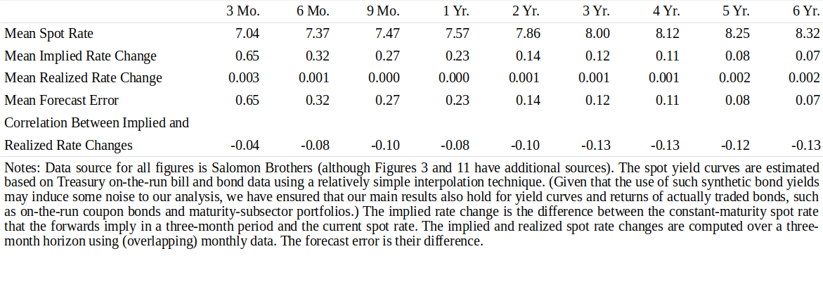
Figure 1 Evaluating the Implied Treasury Forward Yield Curve’s Ability to Predict Actual Rate Changes, 1968-95

Figure 1 shows that, on average, the forwards imply rising rates, especially at short maturities —— simply because the yield curve tends to be upward sloping. However, the rate changes that would offset the yield advantage of longer bonds have not materialized, on average, leading to positive forecast errors. Our unpublished analysis shows that this conclusion holds over longer horizons than three months and over various subsamples, including flat and steep yield curve environments. The fact that the forwards tend to imply too high rate increases is probably caused by positive bond risk premia.

图1显示，平均来说，远期收益率隐含着收益率上涨，特别是在短期端内，这仅仅是因为收益率曲线趋向于向上倾斜。然而，平均而言抵消长期债券收益率优势的收益率变动并没有实现，这导致正的预测误差。我们未发表的分析表明，这个结论在比三个月更长的期间和不同子样本（包括平坦和陡峭的收益率曲线环境）上保持成立。远期收益率倾向于隐含着过高的收益率上涨幅度，这一事实可能是由于正的债券风险溢价的影响。

The last row in Figure 1 shows that the estimated correlations of the implied forward yield changes (or the steepness of the forward rate curve) with subsequent yield changes are negative. These estimates suggest that, if anything, yields tend to move in the opposite direction than that which the forwards imply. Intuitively, small declines in long rates have followed upward-sloping curves, on average, thus augmenting the yield advantage of longer bonds (rather than offsetting it). Conversely, small yield increases have succeeded inverted curves, on average. The big bull markets of the 1980s and 1990s occurred when the yield curve was upward sloping, while the big bear markets in the 1970s occurred when the curve was inverted. We stress, however, that the negative correlations in Figure 1 are quite weak; they are not statistically significant.^[2]

图1的最后一行显示，隐含的远期收益率变化（或远期收益率曲线的陡峭程度）与后续实现的收益率变化的相关性估计为负。这些估计表明，如果有的话，收益率往往会向远期收益率隐含的相反方向变动。直观上来说，平均来看长期收益率的小幅下滑跟随着向上倾斜的曲线，从而增加了长期债券的收益率优势（而不是抵消）。相反，平均而言小幅度的收益率增长跟随倒挂的曲线。1980年代和90年代的大牛市发生在收益率曲线向上倾斜的时期，而1970年代的大熊市在曲线倒挂时发生。然而，我们强调，图1中的负相关性相当弱，没有统计学意义。

Many market participants believe that the bond risk premia are constant over time and that changes in the curve steepness, therefore, reflect shifts in the market's rate expectations. However, the empirical evidence in Figure 1 and in many earlier studies contradicts this conventional wisdom. Historically, steep yield curves have been associated more with high subsequent excess bond returns than with ensuing bond yield increases.^[3]

许多市场参与者认为，债券风险溢价随着时间的推移不发生变化，并且曲线陡峭程度的变化反映了市场收益率预期的变化。然而，图1和许多早期研究中的实证证据与这种传统智慧相矛盾。历史上，陡峭的收益率曲线与随后的债券超额回报更加相关，而不是债券收益率的增长。

One may argue that the historical evidence in Figure 1 is no longer relevant. Perhaps investors forecast yield movements better nowadays, partly because they can express their views more efficiently with easily tradable tools, such as the Eurodeposit futures. Some anecdotal evidence supports this view: Unlike the earlier yield curve inversions, the most recent inversions (1989 and 1995) were quickly followed by declining rates. If market participants actually are becoming better forecasters, subperiod analysis should indicate that the implied forward rate changes have become better predictors of the subsequent rate changes; that is, the rolling correlations between implied and realized rate changes should be higher in recent samples than earlier. In Figure 2, we plot such rolling correlations, demonstrating that the estimated correlations have increased somewhat over the past decade.

人们可能会认为，图1中的历史证据不再可信。也许今天的投资者能更好地预测收益率变动，部分原因是他们可以通过易于交易的工具（如欧洲存款期货）更有效地表达自己的观点。一些轶事证据支持这一观点：与早期的收益率曲线倒挂不同，最近的倒挂（1989年和1995年）发生之后很快出现收益率下降。如果市场参与者实际上正在变成更好的预测者，则子时段分析应该表明隐含的远期收益率变化已经成为后续收益率变化更好的预测因子。也就是说，最近样本中隐含和实现的收益率变化之间的滚动相关性应该比之前高。在图2中，我们绘制了这种滚动相关性，表明在过去十年中估计的相关性有所增加。

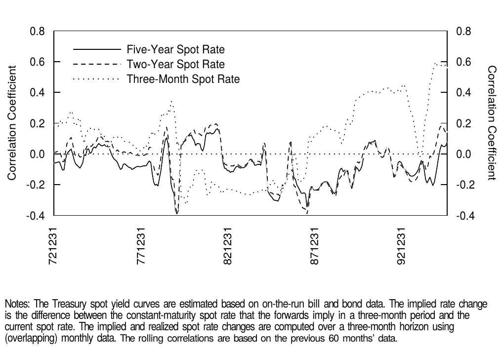
Figure 2 60-Month Rolling Correlations Between the Implied Forward Rate Changes and Subsequent Spot Rate Changes, 1968-95

In Figure 3, we compare the forecasting ability of Eurodollar futures and Treasury bills/notes in the 1987-95 period. The average forecast errors are smaller in the Eurodeposit futures market than in the Treasury market, reflecting the flatter shape of the Eurodeposit spot curve (and perhaps the systematic "richness" of the shortest Treasury bills). In contrast, the correlations between implied and realized rate changes suggest that the Treasury forwards predict future rate changes slightly better than the Eurodeposit futures do. A comparison with the correlations in Figure 1 (the long sample period) shows that the front-end Treasury forwards, in particular, have become much better predictors over time. For the three-month rates, this correlation rises from -0.04 to 0.45, while for the three-year rates, this correlation rises from -0.13 to 0.01. Thus, recent evidence is more consistent with the pure expectations hypothesis than the data in Figure 1, but these relations are so weak that it is too early to tell whether the underlying relation actually has changed. Anyway, even the recent correlations suggest that bonds longer than a year tend to earn their rolling yields.

在图3中，我们比较了欧元美元期货和国库券在1987-95年期间的预测能力。欧洲存款期货市场的平均预测误差小于国债市场，反映了欧洲存款的即期收益率曲线更平坦的形状（也可能是最短期的国库券系统的“高估”预测值）。相比之下，隐含和实现的收益率变化之间的相关性表明，国债远期预测未来收益率变化略好于欧洲存款期货。与图1（长样本期）的相关性的比较表明，前端的国债远期的预测能力随着时间的推移变得更好。对于三月期收益率，这种相关性从-0.04上升到0.45，而对三年期收益率，这种相关性从-0.13上升到0.01。因此，与图1中的数据相比，最近的证据与完全预期假说更为一致，但是这些关系非常弱，判断隐藏的相关性是否真的发生了变化为时尚早。无论如何，即使最近的相关性也表明长于一年的债券往往会获得滚动收益率。

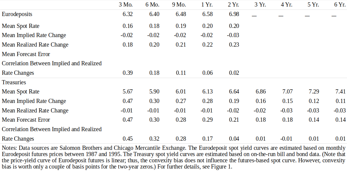
Figure 3 Evaluating the Implied Eurodeposit and Treasury Forward Yield Curve’s Ability to PredictActual Rate Changes, 1987-95

Interpretations

解释

The empirical evidence in Figure 1 is clearly inconsistent with the pure expectations hypothesis.^[4] One possible explanation is that curve steepness mainly reflects time-varying risk premia, and this effect is variable enough to offset the otherwise positive relation between curve steepness and rate expectations. That is, if the market requires high risk premia, the current long rate will become higher and the curve steeper than what the rate expectations alone would imply —— the yield of a long bond initially has to rise so high that it provides the required bond return by its high yield and by capital gain caused by its expected rate decline. In this case, rate expectations and risk premia are negatively related; the steep curve predicts high risk premia and declining long rates. This story could explain the steepening of the front end of the US yield curve in spring 1994 (but not on many earlier occasions when policy tightening caused yield curve flattening).

图1中的实证证据显然与完全预期假说不一致。一个可能的解释是，曲线陡峭程度主要反映了时变的风险溢价，这种影响足够抵消曲线陡峭程度和收益率预期之间原本的正相关性。也就是说，如果市场需要高风险溢价，目前的长期收益率将会变得更高，曲线比单纯的收益率预期隐含的更为陡峭，长期债券的收益率最初必须上涨得很高，才能通过其高收益率及其预期收益率下降所带来的资本回报提供所要求的债券回报。在这种情况下，收益率预期和风险溢价是负相关的；陡峭的曲线预测高风险溢价和长期收益率下降。这可以解释1994年春季美国收益率曲线前端的陡峭（但是在政策收紧导致收益率曲线平坦化的早期情况下，并不是这样）。

The long-run average bond risk premia are positive (see Part 3 of this series and Figure 11 in this report) but the predictability evidence suggests that bond risk premia are time-varying rather than constant. Why should required bond risk premia vary over time? In general, an asset's risk premium reflects the amount of risk and the market price of risk (for details, see Appendix B). Both determinants can fluctuate over time and result in predictability. They may vary with the yield level (rate-level-dependent volatility) or market direction (asymmetric volatility or risk aversion) or with economic conditions. For example, cyclical patterns in required bond returns may reflect wealth-dependent variation in the risk aversion level —— "the cycle of fear and greed."

长期平均债券风险溢价是正的（参见本系列的第3部分和本报告中的图11），但可预测性证据表明债券风险溢价是时变的，而不是恒定的。为什么债券风险溢价随时间而变化？一般来说，资产的风险溢价反映了风险的大小和风险的市场价格（详见附录B）。两个决定因素随着时间的推移可能会波动，并导致可预测性。它们可能随着收益率水平（依赖收益率水平的波动率），或市场方向（不对称的波动率或风险厌恶），或经济状况而变化。例如，债券回报的周期性模式可能反映了风险规避水平中的财富依赖性变化，即“恐惧和贪婪的循环”。

Figure 4 shows the typical business cycle behavior of bond returns and yield curve steepness: Bond returns are high and yield curves are steep near troughs, and bond returns are low and yield curves are flat/inverted near peaks. These countercyclic patterns probably reflect the response of monetary policy to the economy's inflation dynamics, as well as time-varying risk premia (high risk aversion and required risk premia in "bad times" and vice versa). Figure 4 is constructed so that if bonds tend to earn their rolling yields, the two lines are perfectly aligned. However, the graph shows that bonds tend to earn additional capital gains (beyond rolling yields) from declining rates near cyclical troughs —— and capital losses from rising rates near peaks. Thus, realized bond returns are related to the steepness of the yield curve and —— in addition —— to the level of economic activity.

图4显示了债券回报和收益率曲线陡峭程度典型的商业周期行为：债券回报高，收益率曲线在波谷附近陡峭；债券回报低，收益率曲线在峰值附近平坦或倒挂。这些反周期模式可能反映了货币政策对经济通货膨胀的动态反应，以及时变的风险溢价（高风险厌恶和“坏时期”要求的风险溢价，反之亦然）。图4的构造说明，如果债券倾向于获得其滚动收益率，则两条线完全契合。然而，该图表显示，债券往往会从波谷附近的收益率下降中获得额外的资本回报（超出滚动收益率），以及波峰附近的收益率上涨中产生资本损失。因此，实现的债券回报与收益率曲线的陡峭程度相关，并且还与经济活动水平有关。

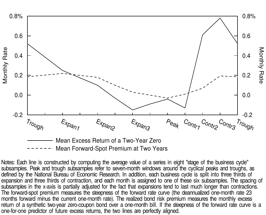
Figure 4 Average Business Cycle Pattern of US Realized Bond Risk Premium and Curve Steepness, 1968-95

These empirical findings motivate the idea that the required bond risk premia vary over time with the steepness of the yield curve and with some other variables. In Part 4 of this series, we show that yield curve steepness indicators and real bond yields, combined with measures of recent stock and bond market performance, are able to forecast up to 10% of the variation in monthly excess bond returns. That is, bond returns are partly forecastable. For quarterly or annual horizons, the predictable part is even larger.^[5]

这些实证结果启发了如下观点，时变的债券风险溢价随着收益率曲线的陡峭程度和其他一些变量而变化。在本系列的第4部分中，我们显示，收益率曲线陡峭程度和实际债券收益率，加上近期股票和债券市场表现的度量，能够预测的月度债券超额回报高达10%。也就是说，债券回报是部分可预测的。对于季度或年度频率的数据，可预测的部分甚至更大。

If market participants are rational, bond return predictability should reflect time-variation in the bond risk premia. Bond returns are predictably high when bonds command exceptionally high risk premia —— either because bonds are particularly risky or because investors are exceptionally risk averse. Bond risk premia may also be high if increased supply of long bonds steepens the yield curve and increases the required bond returns. An alternative interpretation is that systematic forecasting errors cause the predictability. If forward rates really reflect the market's rate expectations (and no risk premia), these expectations are irrational.

如果市场参与者理性，债券回报可预测性应反映债券风险溢价的时变性。当债券风险溢价异常高时（由于债券风险过大，或因为投资者过于规避风险）可以预测债券回报也会高。如果长期债券的供应量增加使收益率曲线更加陡峭，并增加所要求的债券回报，债券风险溢价也可能会很高。另一种解释是系统性的预测错误导致可预测性。如果远期收益率真的反映了市场的收益率预期（没有风险溢价），这些预期是不合理的。

They tend to be too high when the yield curve is upward sloping and too low when the curve is inverted. The market appears to repeat costly mistakes that it could avoid simply by not trying to forecast rate shifts. Such irrational behavior is not consistent with market efficiency. What kind of expectational errors would explain the observed patterns between yield curve shapes and subsequent bond returns? One explanation is a delayed reaction of the market's rate expectations to inflation news or to monetary policy actions. For example, if good inflation news reduces the current short-term rate but the expectations for future rates react sluggishly, the yield curve becomes upward-sloping, and subsequently the bond returns are high (as the impact of the good news is fully reflected in the rate expectations and in the long-term rates).^[6]

当收益率曲线向上倾斜时，它们往往太高，当曲线倒挂时，它们太低。市场似乎重复了昂贵的错误，只能通过不试图预测收益率变动来避免。这种不合理的行为与市场有效性不一致。什么样的预期错误可以解释收益率曲线形状和随后的债券回报之间观察到的模式？一个解释是市场对通货膨胀消息或货币政策行动速度的预期延迟反应。例如，如果利好的通货膨胀消息降低了目前的短期收益率，但对未来收益率的预期反应迟缓，收益率曲线变得向上倾斜，随后债券回报变高（好消息的影响充分反映在收益率预期和长期收益率）。

Because expectations are not observable, we can never know to what extent the return predictability reflects time-varying bond risk premia and systematic forecast errors.^[7] Academic researchers have tried to develop models that explain the predictability as rational variation in required returns. However, yield volatility and other obvious risk measures seem to have little ability to predict future bond returns. In contrast, the observed countercyclic patterns in expected returns suggest rational variation in the risk aversion level —— although they also could reflect irrational changes in the market sentiment. Studies that use survey data to proxy for the market's expectations conclude that risk premia and irrational expectations contribute to the return predictability.

由于预期不可观察，我们永远不知道回报可预测性在多大程度上反映了时变的债券风险溢价和系统预测误差。学术研究人员试图开发模型，将可预测性解释为所要求回报的理性变化。然而，收益率波动率和其他明显的风险度量似乎几乎没有预测未来债券回报的能力。相比之下，预期回报中观察到的反周期模式表明了风险规避水平的理性变化，尽管它们也可以反映市场情绪的非理性变化。使用调查数据代表市场预期的研究得出结论，风险溢价和非理性预期有助于回报可预测性。

Investment Implications

投资实践

If expected bond returns vary over time, historical average returns contain less information about future returns than do indicators of the prevailing economic environment, such as the information in the current yield curve. In principle, the information in the forward rate structure is one of the central issues for fixed-income investors. If the forwards (adjusted for the convexity bias) only reflect the market's rate expectations and if these expectations are unbiased (they are realized, on average), then all government bond strategies would have the same near-term expected return. Yield-seeking activities (convergence trades and relative value trades) would be a waste of time and trading costs. Empirical evidence discussed above suggests that this is not the case: Bond returns are partially predictable, and yield-seeking strategies are profitable in the long run.^[8] However, it pays to use other predictors together with yields and to diversify across various positions, because the predictable part of bond returns is small and uncertain.

如果债券的预期回报随时间而变化，则历史平均回报包含关于未来回报的信息，与当前经济环境的指标（如当前收益率曲线中的信息）相比较少。原则上，远期收益率结构中的信息是固定收益投资者研究的核心问题之一。如果远期收益率（经过凸度偏差调整）仅反映市场的收益率预期，如果这些预期是无偏见的（平均来看将会实现），则所有政府债券策略将具有相同的短期预期回报。追求收益率的活动（如收敛交易和相对价值交易）将是浪费时间和交易成本的。之前的实证证据表明，情况并非如此：债券回报是部分可预测的，长期来看追求收益率的策略是有利可图的。然而，由于债券回报的可预测部分小而且不确定，因此可以将其他预测变量与收益率组合使用或进行分散化投资。

In practice, the key question is perhaps not whether the forwards reflect rate expectations or risk premia but whether actual return predictability exists and who should exploit it. No predictability exists if the forwards (adjusted for the convexity bias) reflect unbiased rate expectations. If predictability exists and is caused by expectations that are systematically wrong, everyone can exploit it. If predictability exists and is caused by rational variation in the bond risk premia, only some investors should take advantage of the opportunities to enhance long-run average returns; many others would find higher expected returns in "bad times" no more than a fair compensation for the greater risk or the higher risk aversion level. Only risk-neutral investors and atypical investors whose risk perception and risk tolerance does not vary synchronously with those of the market would want to exploit any profit opportunities —— and these investors would not care whether rationally varying risk premia or the market's systematic forecast errors cause these opportunities.

在实践中，关键问题可能不在于远期收益率是否反映收益率预期或风险溢价，而是实际回报可预测性是否存在，谁应该利用它。如果远期收益率（经过凸度偏差调整）反映了无偏的收益率预期，则不存在可预测性。如果可预测性存在并且是由系统性错误的预期引起的，每个人都可以利用它。如果存在可预测性，是由债券风险溢价的合理变动引起的，只有一些投资者能利用机会增加长期平均回报；许多其他人会在“坏时期”中找到更高的预期回报，而不是为更大的风险或更高的风险规避水平提供公平的补偿。只有风险中性的投资者和不典型的投资者，他们的风险感知和风险承受能力与市场上的人不同步，他们会想要利用任何利润机会，而这些投资者不会关心理性的风险溢价或市场的系统性预测错误是否会带来这些机会。

HOW SHOULD WE INTERPRET THE YIELD CURVE CURVATURE?

如何解释收益率曲线的曲率

The market's curve reshaping expectations, volatility expectations and expected return structure determine the curvature of the yield curve. Expectations for yield curve flattening imply expected profits for duration-neutral long-barbell versus short-bullet positions, tending to make the yield curve concave (thus, the yield disadvantage of these positions offsets their expected profits from the curve flattening). Expectations for higher volatility increase the value of convexity and the expected profits of these barbell-bullet positions, again inducing a concave yield curve shape. Finally, high required returns of intermediate bonds (bullets) relative to short and long bonds (barbells) makes the yield curve more concave. Conversely, expectations for yield curve steepening or for low volatility, together with bullets' low required returns, can even make the yield curve convex.

市场曲线形变预期、波动率预期和预期回报结构决定了收益率曲线的曲率。收益率曲线平坦化的预期意味着久期中性的多杠铃-空子弹组合的预期利润，倾向于使收益率曲线上凸（因此，这些头寸的收益率劣势抵消了其曲线平坦化带来的预期利润）。高波动率的预期增加了杠铃-子弹组合的凸度价值和预期利润，再次导致了收益率曲线上凸的形状。最后，相对于短期和长期债券（杠铃组合），市场对中期债券（子弹组合）要求的高回报使收益率曲线更上凸。相反，对于收益率曲线变陡或低波动率的预期，以及对子弹组合要求的低回报，甚至可以使收益率曲线下凸。

In this section, we analyze the yield curve curvature and focus on two key questions: (1) How important are each of the three determinants in changing the curvature over time?; and (2) why is the long-run average shape of the yield curve concave?

在本节中，我们分析收益率曲线的曲率，并重点关注两个关键问题：（1）三个决定因素在改变曲率中的重要性分别是多少？和（2）为什么长期平均来看收益率曲线的形状是上凸的？

Empirical Evidence

实证证据

Some earlier studies suggest that the curvature of the yield curve is closely related to the market's volatility expectations, presumably due to the convexity bias. However, our empirical analysis indicates that the curvature varies more with the market's curve-reshaping expectations than with the volatility expectations. The broad curvature of the yield curve varies closely with the steepness of the curve, probably reflecting mean-reverting rate expectations.

一些较早的研究表明，收益率曲线的曲率与市场的波动率预期密切相关，推测是由于凸度偏差。然而，我们的实证分析表明，曲率更倾向于随着市场的曲线形变预期而不是波动率预期变化。收益率曲线的曲率大致紧随曲线的陡峭程度变化，可能反映了均值回归的收益率预期。

Figure 5 plots the Treasury spot curve when the yield curve was at its steepest and at its most inverted in recent history and on a date when the curve was extremely flat. This graph suggests that historically low short rates have been associated with steep yield curves and high curvature (concave shape), while historically high short rates have been associated with inverted yield curves and negative curvature (convex shape).

图5绘制了当近期历史中收益率曲线最陡峭、最倒挂以及最平坦的国债即期收益率曲线。该图表明，历史上低的短期收益率与陡峭的收益率曲线和高曲率（上凸）相关联，而历史上高的短期收益率与倒挂的收益率曲线和负曲率（下凸）相关联。

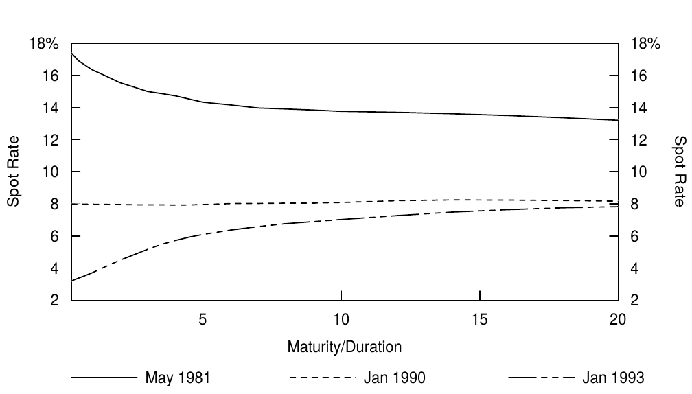
Figure 5 Treasury Spot Yield Curves in Three Environments

The correlation matrix of the monthly changes in yield levels, curve steepness and curvature in Figure 6 confirms these relations. Steepness measures are negatively correlated with the short rate levels (but almost uncorrelated with the long rate levels), reflecting the higher likelihood of bull steepeners and bear flatteners than bear steepeners and bull flatteners. However, we focus on the high correlation (0.79) between the changes in the steepness and the changes in the curvature. This relation has a nice economic logic. Our curvature measure can be viewed as the yield carry of a curve-steepening position, a duration-weighted bullet-barbell position (long a synthetic three-year zero and short equal amounts of a three-month zero and a 5.75-year zero). If market participants have mean-reverting rate expectations, they expect yield curves to revert to a certain average shape (slightly upward sloping) in the long run. Then, exceptionally steep curves are associated with expectations for subsequent curve flattening and for capital losses on steepening positions. Given the expected capital losses, these positions need to offer an initial yield pickup, which leads to a concave (humped) yield curve shape. Conversely, abnormally flat or inverted yield curves are associated with the market's expectations for subsequent curve steepening and for capital gains on steepening positions. Given the expected capital gains, these positions can offer an initial yield giveup, which induces a convex (inversely humped) yield curve.

图6中收益率水平、曲线陡峭程度和曲率月度变化的相关矩阵证实了这些关系。陡峭程度与短期收益率水平呈负相关（但与长期收益率水平几乎无关），反映出陡峭程度与牛陡和熊平而不是牛平和熊斗之间更高的相关性。然而，我们专注于陡峭程度变化和曲率变化之间的高相关性（0.79）。这种关系有一个很好的经济逻辑。我们的曲率可以看作是做陡曲线头寸的收益率Carry，即久期加权的子弹-杠铃组合（做多三年期零息债券和做空等量的三月期零息债券和5.75年期零息债券）。如果市场参与者具有均值回归的收益率预期，那么长期来看，他们预期收益率曲线将恢复到一定的平均形状（略向上倾斜）。然后，非常陡峭的曲线与后续曲线平坦化的预期和做陡头寸的资本损失相关。鉴于预期的资本损失，这些头寸需要提供初始的收益率补偿，这导致了上凸（隆起）的收益率曲线形状。相反，异常平坦或倒挂的收益率曲线与市场对随后曲线陡峭的预期和做陡头寸的资本回报有关。鉴于预期的资本回报，这些头寸可以提供初始收益率损失，这会产生一个下凸（向下隆起）的收益率曲线。

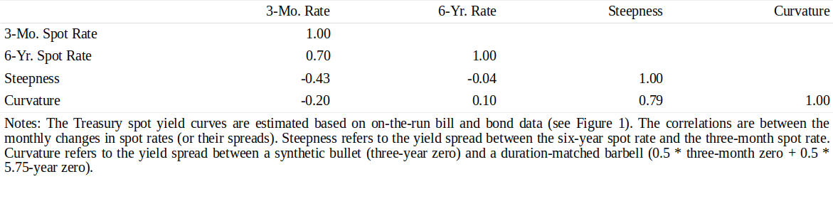
Figure 6 Correlation Matrix of Yield Curve Level, Steepness and Curvature, 1968-95

Figure 7 illustrates the close comovement between our curve steepness and curvature measures. The mean-reverting rate expectations described above are one possible explanation for this pattern. Periods of steep yield curves (mid-1980s and early 1990s) are associated with high curvature and, thus, a large yield pickup for steepening positions, presumably to offset their expected losses as the yield curve flattens. In contrast, periods of flat or inverted curves (1979-81, 1989-90 and 1995) are associated with low curvature or even an inverse hump. Thus, barbells can pick up yield and convexity over duration-matched bullets, presumably to offset their expected losses when the yield curve is expected to steepen toward its normal shape.

图7示出了我们的曲线陡峭程度和曲率之间的紧密联系。上述均值回归的收益率预期是这种模式的一个可能解释。陡峭收益率曲线的时期（1980年代中期和90年代初）与高曲率相关，因此，对于做陡头寸而言，大量的收益率补偿可能抵消了随后收益率曲线变平的预期损失。相比之下，平坦或倒挂曲线的时期（1979-81,1989-90和1995）与低曲率甚至下凸相关。因此，杠铃组合相对于久期匹配的子弹组合有收益率和凸度优势，当预期收益率曲线朝向其正常形状而变陡峭时，可以抵消其预期的损失。

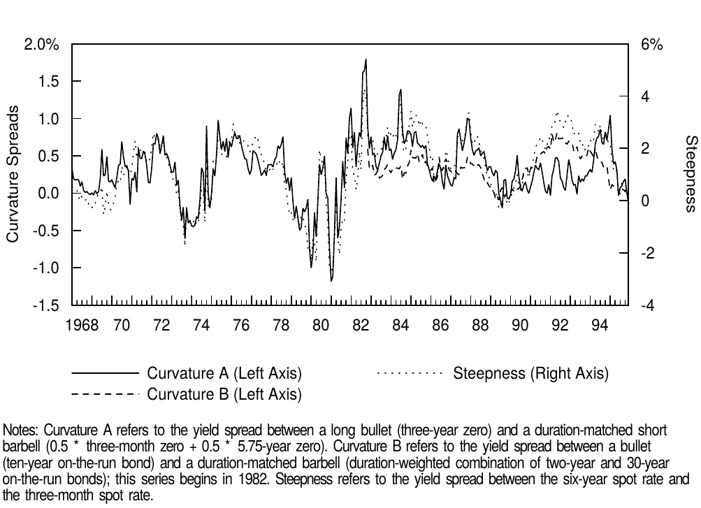
Figure 7 Curvature and Steepness of the Treasury Curve, 1968-95

The expectations for mean-reverting curve steepness influence the broad curvature of the yield curve. In addition, the curvature of the front end sometimes reflects the market's strong view about near-term monetary policy actions and their impact on the curve steepness. Historically, the Federal Reserve and other central banks have tried to smooth interest rate behavior by gradually adjusting the rates that they control. Such a rate-smoothing policy makes the central bank's actions partly predictable and induces a positive autocorrelation in short-term rate behavior. Thus, if the central bank has recently begun to ease (tighten) monetary policy, it is reasonable to expect the monetary easing (tightening) to continue and the curve to steepen (flatten).

曲线陡峭程度均值回归的预期影响了大部分收益率曲线的曲率。此外，曲线前端的曲率有时反映了市场对近期货币政策行动及其对曲线陡峭程度影响的强烈观点。历史上，美联储等央行已经试图通过逐步调整收益率来平滑收益率行为。这种收益率平滑政策使中央银行的行为部分可预测，并导致短期收益率行为正的自相关性。因此，如果中央银行最近开始放松（收紧）货币政策，可以合理地预期货币宽松政策（紧缩）将继续，曲线将变陡峭（平坦）。

In the earlier literature, the yield curve curvature has been mainly associated with the level of volatility. Litterman, Scheinkman and Weiss ("Volatility and the Yield Curve," Journal of Fixed Income, 1991) pointed out that higher volatility should make the yield curve more humped (because of convexity effects) and that a close relation appeared to exist between the yield curve curvature and the implied volatility in the Treasury bond futures options. However, Figure 8 shows that the relation between curvature and volatility was close only during the sample period of the study (1984-88). Interestingly, no recessions occurred in the mid-1980s, the yield curve shifts were quite parallel and the flattening/steepening expectations were probably quite weak. The relation breaks down before and after the 1984-88 period, especially near recessions, when the Fed is active and the market may reasonably expect curve reshaping. For example, in 1981 yields were very volatile but the yield curve was convex (inversely humped); see Figures 5 and 13. It appears that the market's expectations for future curve reshaping are more important determinants of the yield curve curvature than are its volatility expectations (convexity bias). The correlations of our curvature measures with the curve steepness are around 0.8 while those with the implied option volatility are around 0.1. Therefore, it is not surprising that the implied volatility estimates that are based on the yield curve curvature are not closely related to the implied volatilities that are based on option prices. Using the yield curve shape to derive implied volatility can result in negative volatility estimates; this unreasonable outcome occurs in simple models when the expectations for curve steepening make the yield curve inversely humped (see Part 5 of this series).

在早期的文献中，收益率曲线曲率主要与波动率水平有关。Litterman，Scheinkman 和 Weiss 指出（《Volatility and the Yield Curve》，Journal of Fixed Income，1991），较高的波动率应使收益率曲线更加上凸（由于凸度效应），并且收益率曲线曲率和国债期货期权的隐含波动率之间存在着密切的关系。然而，图8显示，曲率和波动率之间的关系仅存在于研究的样本期间（1984-88）。有趣的是，1980年代中期没有发生经济衰退，收益率曲线变化同步性相当高，变平或变陡的预期可能相当薄弱。这种关系在1984-88年度之前和之后不成立，尤其是在近期的经济衰退时期，这时美联储活跃，市场理性的预期曲线形变。例如，1981年的收益率波动率非常大，但收益率曲线是下凸的（向下隆起），见图5和图13。似乎市场对未来曲线形变的预期是收益率曲线曲率的重要决定因素，而不是其波动率预期（凸度偏差）。我们测算的曲率与曲线陡峭程度的相关性约为0.8，而与期权隐含波动率的相关性约为0.1。因此，基于收益率曲线曲率的隐含波动率估计与基于期权价格的隐含波动率并不密切相关。使用收益率曲线形状导出隐含波动率可导致负的波动率估计，这种不合理的结果发生在简单的模型中，当曲线变陡峭的预期使得收益率曲线向下隆起时（见本系列的第5部分）。

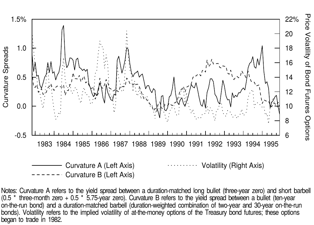
Figure 8 Curvature and Volatility in the Treasury Market, 1982-95

Now we move to the second question "Why is the long-run average shape of the yield curve concave?" Figure 9 shows that the average par and spot curves have been concave over our 28-year sample period.^[9] Recall that the concave shape means that the forwards have, on average, implied yield curve flattening (which would offset the intermediate bonds' initial yield advantage over duration-matched barbells). Figure 10 shows that, on average, the implied flattening has not been matched by sufficient realized flattening. Not surprisingly, flattenings and steepenings tend to wash out over time, whereas the concave spot curve shape has been quite persistent. In fact, a significant positive correlation exists between the implied and the realized curve flattening, but the average forecast errors in Figure 10 reveal a bias of too much implied flattening. This conclusion holds when we split the sample into shorter subperiods or into subsamples of a steep versus a flat yield curve environment or a rising-rate versus a falling-rate environment.

现在我们转到第二个问题：“为什么收益率曲线的长期平均形状是上凸的？”图9显示，在28年的样本周期内，平均到期和即期收益率曲线均呈上凸。回想一下，上凸形意味着，平均来看远期收益率隐含着收益率曲线变平（这将抵消中期债券相对于久期匹配的杠铃组合的初始收益率优势）。图10显示，平均而言，隐含的平坦化并没有被充分实现。毫不奇怪，变平和变陡倾向于随着时间的推移而逐渐消失，但上凸即期收益率曲线的形状已经相当持久。事实上，隐含和实现的曲线平坦化之间存在显着的正相关，但图10中的平均预测误差揭示了过于隐含平坦化的偏差。当我们将样本依据陡峭与平坦或收益率上升与下降的情形分解成子样本时，这一结论是成立的。

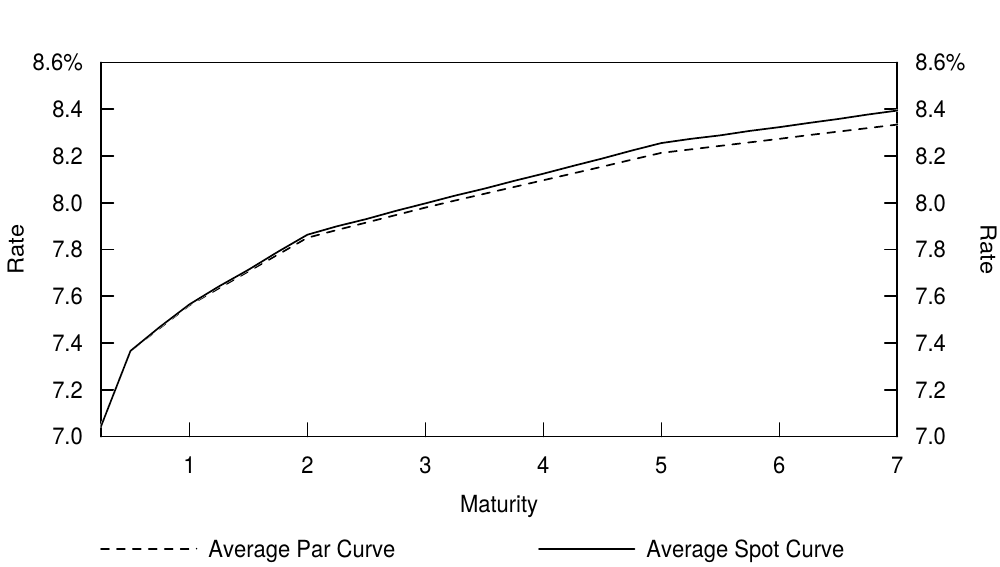
Figure 9 Average Yield Curve Shape, 1968-95

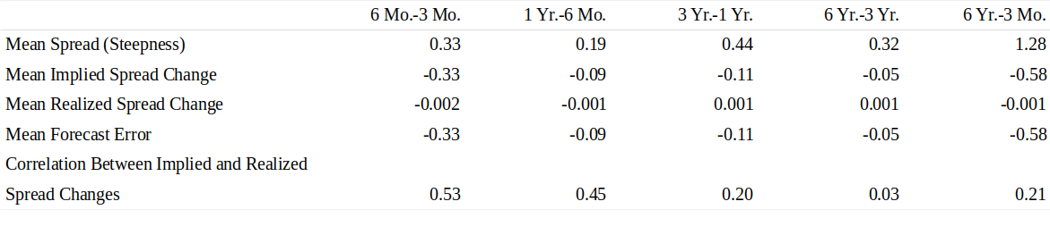
Figure 10 Evaluating the Implied Forward Yield Curve’s Ability to Predict Actual Changes in the Spot Yield Curve’s Steepness, 1968-95

Figure 10 shows that, on average, the capital gains caused by the curve flattening have not offset a barbell's yield disadvantage (relative to a duration-matched bullet). A more reasonable possibility is that the barbell's convexity advantage has offset its yield disadvantage. We can evaluate this possibility by examining the impact of convexity on realized returns over time. Empirical evidence suggests that the convexity advantage is not sufficient to offset the yield disadvantage (see Figure 12 in Part 5 of this series). Alternatively, we can examine the shape of historical average returns because the realized returns should reflect the convexity advantage. This convexity effect is certainly a partial explanation for the typical yield curve shape —— but it is the sole effect only if duration-matched barbells and bullets have the same expected returns. Equivalently, if the required bond risk premium increases linearly with duration, the average returns of duration-matched barbells and bullets should be the same over a long neutral period (because the barbells' convexity advantage exactly offsets their yield disadvantage). The average return curve shape in Figure 1, Part 3 and the average barbell-bullet returns in Figure 11, Part 5 suggest that bullets have somewhat higher long-run expected returns than duration-matched barbells. We can also report the historical performance of synthetic zero positions over the 1968-95 period: The average annualized monthly return of a four-year zero is 9.14%, while the average returns of increasingly wide duration-matched barbells are progressively lower (3-year and 5-year 9.05%, 2-year and 6-year 9.00%, 1-year and 7-year 8.87%). Overall, the typical concave shape of the yield curve likely reflects the convexity bias and the concave shape of the average bond risk premium curve rather than systematic flattening expectations, given that the average flattening during the sample is zero.

图10显示，平均来说，曲线平坦化引起的资本回报并未抵消杠铃组合的收益率劣势（相对于久期匹配的子弹组合）。更合理的可能性是，杠铃组合的凸度优势抵消了其收益率劣势。我们可以通过检查凸度对实际回报的影响来评估这种可能性。经验证据表明，凸度优势不足以抵消收益率劣势（参见本系列第5部分的图12）。或者，我们可以检查历史平均回报的形状，因为实现的回报应该反映凸度优势。这种凸度效应当然是对典型收益率曲线形状的部分解释，但只有久期匹配的杠铃组合和子弹组合具有相同的预期回报，才是唯一的效果。同样地，如果债券风险溢价随久期线性增长，久期匹配的杠铃组合和子弹组合的平均回报在长时间的中性时期应该是相同的（因为杠铃组合的凸度优势恰好抵消了他们的收益率劣势）。第3部分图1的平均回报曲线形状以及第5部分图11中的平均杠铃-子弹组合回报表明，子弹组合比久期匹配的杠铃组合具有较高的长期预期回报。我们还指出1968-95年期间合成零息债券头寸的历史表现：4年期零息债券的平均年化月度回报为9.14%，而久期匹配的杠铃组合的平均回报逐渐下降（3-5年期组合为9.05%，2-6年期组合为9.00%，1-7年期组合为8.87%）。总体而言，考虑到样本中平均来看曲线平坦的比例为零，收益率曲线典型的上凸形态可能反映了凸度偏差和债券风险溢价曲线的上凸形态，而不是系统的曲线变平预期。

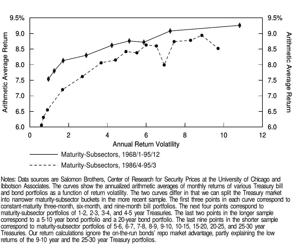
Figure 11 Average Treasury Maturity-Subsector Returns as a Function of Return Volatility

Interpretations

解释

The impact of curve reshaping expectations and convexity bias on the yield curve shape are easy to understand, but the concave shape of the bond risk premium curve is more puzzling. In this subsection, we explore why bullets should have a mild expected return advantage over duration-matched barbells. One likely answer is that duration is not the relevant risk measure. However, we find that average returns are concave even in return volatility, suggesting a need for a multi-factor risk model. We first discuss various risk-based explanations in detail and then consider some alternative "technical" explanations for the observed average return patterns.

曲线形变预期和凸度偏差对收益率曲线形状的影响很容易理解，但债券风险溢价曲线的上凸形态更令人困惑。在本小节中，我们探讨为什么子弹组合应该比久期匹配的杠铃组合具有微弱的预期回报优势。一个可能的答案是，久期不是有意义的风险度量。然而，我们发现即使作为回报波动率的函数平均回报也是上凸的，这表明需要一个多因子风险模型。我们首先详细讨论各种基于风险的解释，然后考虑观察到的均值回归模式的替代“技术性”解释。

All one-factor term structure models imply that expected returns should increase linearly with the bond's sensitivity to the risk factor. Because these models assume that bond returns are perfectly correlated, expected returns should increase linearly with return volatility (whatever the risk factor is). However, bond durations are proportional to return volatilities only if all bonds have the same basis-point yield volatilities. Perhaps the concave shape of the average return-duration curve is caused by (i) a linear relation between expected return and return volatility and (ii) a concave relation between return volatility and duration that, in turn, reflects an inverted or humped term structure of yield volatility (see Figure 15). Intuitively, a concave relation between the actual return volatility and duration would make a barbell a more defensive (bearish) position than a duration-matched bullet. The return volatility of a barbell is simply a weighted average of its constituents' return volatilities (given the perfect correlation); thus, the barbell's volatility would be lower than that of a duration-matched bullet.

所有单因子期限结构模型认定预期回报随着债券对风险因子的敏感性而线性增长。因为这些模型假设债券回报完全相关，所以预期回报应随回报波动率线性增加（无论风险因子如何）。然而，只有所有债券具有相同的基点收益率波动率，债券久期才与回报波动率成比例。平均回报-久期曲线的上凸形状也许是由（i）预期回报和回报波动率之间的线性关系引起的；（ii）回报波动率与久期之间的上凸关系，反过来又反映了一个倒挂或隆起的收益率波动率期限结构（见图15）。直觉上，实际回报波动率与久期之间的上凸关系将使杠铃组合比久期匹配的子弹组合更具防守（看跌）性。杠铃组合的回报波动率只是其成分回报波动率的加权平均值（给定完美的相关性）；因此，杠铃组合的波动率将低于久期匹配的子弹组合。

Figures 13 and 14 will demonstrate that the empirical term structure of yield volatility has been inverted or humped most of the time. Thus, perhaps a barbell and a bullet with equal return volatilities (as opposed to equal durations) should have the same expected return. However, it turns out that the bullet's return advantage persists even when we plot average returns on historical return volatilities. Figure 11 shows the historical average returns of various maturity-subsector portfolios of Treasury bonds as a function of return volatility. The average returns are based on two relatively neutral periods, January 1968 to December 1995 and April 1986 to March 1995. We still find that the average return curves have a somewhat concave shape. Note that we demonstrate the concave shape in a conservative way by graphing arithmetic average returns; the geometric average return curves would be even more concave.^[10]

图13和14将证明大部分时间内收益率波动率的经验性期限结构是倒挂或隆起的。因此，也许杠铃组合和子弹组合具有相等的回报波动率（而不是相等的久期）才具有相同的预期回报。然而，事实证明，即使我们绘制平均回报关于历史回报波动率的变化，子弹组合的回报优势仍然存在。图11显示了国债各种期限投资组合的历史平均回报（作为回报波动率的函数）。平均回报基于1968年1月至1995年12月和1986年4月至1995年3月的两个相对中性的时期。我们仍然发现平均收益率曲线有一些上凸。注意，通过绘制算术平均回报，我们以保守的方式展示上凸形状；几何均值收益率曲线将更加上凸。

As explained above, one-factor term structure models assume that bond returns are perfectly correlated. One-factor asset pricing models are somewhat more general. They assume that realized bond returns are influenced by only one systematic risk factor but that they also contain a bond-specific residual risk component (which can make individual bond returns imperfectly correlated). Because the bond-specific risk is easily diversifiable, only systematic risk is rewarded in the marketplace. Therefore, expected returns are linear in the systematic part of return volatility. This distinction is not very important for government bonds because their bond-specific risk is so small. If we plot the average returns on systematic volatility only, the front end would be slightly less steep than in Figure 11 because a larger part of short bills' return volatility is asset-specific. Nonetheless, the overall shape of the average return curve would remain concave.

如上所述，单因子期限结构模型假定债券回报完全相关。单因子资产定价模式更为一般化。他们假定实现的债券回报只受一个系统风险因子的影响，但也包含一个特定于债券的剩余风险成分（可以使个别债券回报不完全相关）。由于债券特定风险易于分散，因此只有系统风险才能在市场上得到回报。因此，预期回报关于回报波动率中对应系统风险的部分是线性的。这种区别对于政府债券来说不是很重要，因为它们的债券特定风险很小。如果我们仅绘制平均收益率关于系统波动率的关系，图11中前端将略低，因为较大部分短期国库券的回报波动率是因资产而异。然而，平均收益率曲线的整体形状将保持上凸。

Convexity bias and the term structure of yield volatility explain the concave shape of the average yield curve partly, but a nonlinear expected return curve appears to be an additional reason. Figure 11 suggests that expected returns are somewhat concave in return volatility. That is, long bonds have lower required returns than one-factor models imply. Some desirable property in the longer cash flows makes the market accept a lower expected excess return per unit of return volatility for them than for the intermediate cash flows. We need a second risk factor, besides the rate level risk, to explain this pattern. Moreover, this pattern may teach us something about the nature of the second factor and about the likely sign of its risk premium. We will next discuss heuristically two popular candidates for the second factor —— interest rate volatility and yield curve steepness. We further discuss the theoretical determinants of required risk premia in Appendix B.

凸度偏差和收益率波动率的期限结构部分解释了平均收益率曲线的上凸形状，但非线性预期收益率曲线似乎是一个额外的原因。图11表明，预期回报关于回报波动率有些上凸。也就是说，长期债券的所要求的回报要低于单因子模型所隐含的。较中期现金流而言，长期现金流的一些有利特性使得市场愿意接受单位回报波动率上较低的预期超额回报。除了收益率水平的风险，我们需要第二个风险因子以解释这种模式。此外，这种模式可能会告诉我们关于第二个因子的性质和风险溢价的可能符号。我们接下来讨论第二个因子的两个流行选项，收益率波动率和收益率曲线陡峭程度。我们在附录B中进一步讨论风险溢价的理论决定因素。

Volatility as the second factor could explain the observed patterns if the market participants, in the aggregate, prefer insurance-type or "long-volatility" payoffs. Even nonoptionable government bonds have an option like characteristic because of the convex shape of their price-yield curves. As discussed in Part 5 of this series, the value of convexity increases with a bond's convexity and with the perceived level of yield volatility. If the volatility risk is not "priced" in expected returns (that is, if all "delta-neutral" option positions earn a zero risk premium), a yield disadvantage should exactly offset longer bonds' convexity advantage. However, the concave shape of the average return curve in Figure 11 suggests that positions that benefit from higher volatility have lower expected returns than positions that are adversely affected by higher volatility. Although the evidence is weak, we find the negative sign for the price of volatility risk intuitively appealing. The Treasury market participants may be especially averse to losses in high-volatility states, or they may prefer insurance-type (skewed) payoffs so much that they accept lower long-run returns for them.^[11] Thus, the long bonds' low expected return could reflect the high value many investors assign to positive convexity. However, because short bonds exhibit little convexity, other factors are needed to explain the curvature at the front end of the yield curve.

波动率作为第二个因子可以解释观察到的模式，如果市场参与者总体上偏好保险类型或“做多波动率”的回报。即使不嵌入期权的政府债券也有一个期权特征，因为它们的价格-收益率曲线是下凸的形状。如本系列第5部分所述，凸度价值随着债券的凸度和收益率波动率的感知水平而增加。如果波动率风险在预期回报中没有“定价”（也就是说，如果所有“delta中性”期权头寸都获得零风险溢价），收益率劣势应该恰好抵消较长期债券的凸度优势。然而，图11中平均收益率曲线的上凸形状表明，受益于较高波动率头寸的预期回报低于受制于较高波动率影响的头寸。虽然证据薄弱，但我们发现负的波动率风险价格在直觉上是有吸引力的。国债市场参与者可能特别反对高波动率状态的损失，或者他们可能更喜欢保险型（有偏）的回报，以至于他们接受较低的长期回报。因此，长期债券的低预期回报可能反映出许多投资者给予正凸度的高价值。然而，由于短债券表现出很小的凸度，因此需要其他因素来解释收益率曲线前端的曲率。

Yield curve steepness as the second factor (or short rate and long rate as the two factors) could explain the observed patterns if curve-flattening positions tend to be profitable just when investors value them most. We do not think that the curve steepness is by itself a risk factor that investors worry about, but it may tend to coincide with a more fundamental factor. Recall that the concave average return curve suggests that self-financed curve-flattening positions have negative expected returns —— because they are more sensitive to the long rates (with low reward for return volatility) than to the short/intermediate rates (with high reward for return volatility). This negative risk premium can be justified theoretically if the flattening trades are especially good hedges against "bad times." When asked what constitutes bad times, an academic's answer is a period of high marginal utility of profits, while a practitioner's reply probably is a deep recession or a bear market. The empirical evidence on this issue is mixed. It is clear that long bonds performed very well in deflationary recessions (the United States in the 1930s, Japan in the 1990s). However, they did not perform at all well in the stagflations of the 1970s when the predictable and realized excess bond returns were negative. Since the World War II, the US long bond performance has been positively correlated with the stock market performance —— although bonds turned out to be a good hedge during the stock market crash of October 1987. Turning now to flattening positions, these have not been good recession hedges either; the yield curves typically have been flat or inverted at the beginning of a recession and have steepened during it (see also Figure 4).^[12] Nonetheless, flattening positions typically have been profitable in a rising rate environment; thus, they have been reasonable hedges against a bear market for bonds.

作为第二个因子的收益率曲线陡峭程度（或者短期和长期收益率作为两个因素）可以解释观察到的模式，只有当投资者看重时，做平曲线的头寸才会有利可图。我们不认为曲线陡峭程度本身就是投资者担心的风险因子，但它可能倾向于与更根本的因素相吻合。回想一下，平均来看上凸的收益率曲线表明，自融资的做平曲线头寸具有负的预期回报，因为它们对长期收益率（回报波动率的回报较低）比对短期或中期收益率（回报波动率的回报较高）更敏感。理论上这个负的风险溢价可以是合理的，如果做平交易是对“坏时期”特别好的对冲。当被问及什么是坏时期时，学术界的答案是利润的高边际效用时期，而从业者的回答可能是严重衰退期或熊市。关于这个问题的经验证据是混合的。很明显，长期债券在通货紧缩的衰退期（1930年代的美国，1990年代的日本）中表现良好。然而，当可预测和实现的债券超额回报为负数时，它们在1970年代的困境中表现不佳。自二次大战以来，美国长期债券表现与股市表现呈正相关，尽管在1987年10月的股市崩盘期间债券成为良好的对冲。现在转向做平头寸，这些衰退对冲表现并不好，收益率曲线通常在经济衰退开始时已经平坦或倒挂，并在其期间陡峭（参见图4）。尽管如此，做平的头寸通常在收益率上涨的环境中是有利可图的。因此，他们对债券市场进行了合理的对冲。

We conclude that risk factors that are related to volatility or curve steepness could perhaps explain the concave shape of the average return curve —— but these are not the only possible explanations. "Technical" or "institutional" explanations include the value of liquidity (the ten-year note and the 30-year bond have greater liquidity and lower transaction costs than the 11-29 year bonds, and the on-the-run bonds can earn additional income when they are "special" in the repo market), institutional preferences (immunizing pension funds may accept lower yield for "riskless" long-horizon assets, institutionally constrained investors may demand the ultimate safety of one-month bills at any cost, fewer natural holders exist for intermediate bonds), and the segmentation of market participants (the typical short-end holders probably tolerate return volatility less well than do the typical long-end holders, which may lead to a higher reward for duration extension at the front end).^[13]

我们得出结论，与波动率或曲线陡峭程度相关的风险因子可能解释了平均回报曲线的上凸形状，但这并不是唯一可能的解释。“技术性”或“制度性”解释包括流动性的价值（10年期债券和30年期债券的流动性更大，交易成本比11-29年期债券低，当活跃债券在回购市场被“特殊”对待时，可以赚取额外收入）、机构偏好（养老基金可能会接受较低回报的“无风险”长期资产，制度上受限制的投资者可能要求不惜成本的保障一月期国库券的最终安全，中期债券存在较少的自然持有人）、市场参与者的分割（典型的短期持有者可能不如长期持有者更能忍受回报波动率，这可能会导致在曲线前端延长久期能获得更高回报）。

Investment Implications

投资应用

Bullets tend to outperform barbells in the long run, although not by much. It follows that as a long-run policy, it might be useful to bias the investment benchmarks and the core Treasury holdings toward intermediate bonds, given any duration. In the short run, the relative performance of barbells and bullets varies substantially —— and mainly with the yield curve reshaping. Investors who try to "arbitrage" between the volatility implied in the curvature of the yield curve and the yield volatility implied in option prices will find it very difficult to neutralize the inherent curve shape exposure in these trades. An interesting task for future research is to study how well barbells' and bullets' relative short-run performance can be forecast using predictors such as the yield curve curvature (yield carry), yield volatility (value of convexity) and the expected mean reversion in the yield spread.

从长远来看，子弹组合往往跑赢杠铃组合，虽然不算太多。因此，作为长期策略策，在任何期限内将投资基准和持有的核心国债偏向于中期债券可能是有用的。在短期内，杠铃组合和子弹组合的相对表现差异很大，主要是收益率曲线形变导致。投资者试图在收益率曲线曲率隐含的波动率与期权价格中隐含的收益率波动率之间“套利”，将很难中和这些交易中固有的曲线形状敞口。未来研究的一个有趣的任务是研究如何使用预测因子，诸如收益率曲线曲率（收益率 Carry）、收益率波动率（凸度价值）和利差的预期均值回归，来预测杠铃组合和子弹组合的相对短期表现。

HOW DOES THE YIELD CURVE EVOLVE OVER TIME?

收益率曲线如何随时间变化

The framework used in the series Understanding the Yield Curve is very general; it is based on identities and approximations rather than on economic assumptions. As discussed in Appendix A, many popular term structure models allow the decomposition of forward rates into a rate expectation component, a risk premium component, and a convexity bias component. However, various term structure models make different assumptions about the behavior of the yield curve over time. Specifically, the models differ in their assumptions regarding the number and identity of factors influencing interest rates, the factors' expected behavior (the degree of mean reversion in short rates and the role of a risk premium) and the factors' unexpected behavior (for example, the dependency of yield volatility on the yield level). In this section, we describe some empirical characteristics of the yield curve behavior that are relevant for evaluating the realism of various term structure models.^[14] In Appendix A, we survey other aspects of the term structure modeling literature. Our literature references are listed after the appendices; until then we refer to these articles by author's name.

《理解收益率曲线》系列中使用的框架非常通用，是基于确定性和近似而不是经济假设。如附录A所述，许多流行的期限结构模型允许将远期收益率分解为收益率预期部分、风险溢价部分和凸度偏差部分。然而，各种期限结构模型对收益率曲线随时间的行为做出不同的假设。具体来说，这些模型的差异在于影响收益率的因子的数量和特性、因子的预期行为（短期收益率均值回归的程度和风险溢价的作用）以及因子的非预期行为（例如，收益率波动率对收益率水平的依赖）。在本节中，我们描述与评估与各种期限结构模型相关的若干收益率曲线行为经验特征。在附录A中，我们对期限结构模型文献的其他方面进行了综述。我们的参考文献列在附录之后，我们以作者的名字来引用这些文章。

The simple model of only parallel shifts in the spot curve makes extremely restrictive and unreasonable assumptions —— for example, it does not preclude negative interest rates.^[15] In fact, it is equivalent to the Vasicek (1977) model with no mean reversion. All one-factor models imply that rate changes are perfectly correlated across bonds. The parallel shift assumption requires, in addition, that the basis-point yield volatilities are equal across bonds. Other one-factor models may imply other (deterministic) relations between the yield changes across the curve, such as multiplicative shifts or greater volatility of short rates than of long rates. Multi-factor models are needed to explain the observed imperfect correlations across bonds —— as well as the nonlinear shape of expected bond returns as a function of return volatility that was discussed above.

在即期收益率曲线上只有平行偏移的简单模型，构成限制极大和不合理的假设，例如，它不排除负收益率。事实上，它相当于没有均值回归的 Vasicek（1977）模型。所有单因子模型意味着收益率变化在债券之间完全相关。平行偏移假设另外要求基点收益率波动率在债券之间是相等的。其他单因子模型可能存在着曲线上的收益率变化之间的其他（确定性）关系，如可乘性偏移或短期收益率波动率大于长期收益率。需要多因子模型来解释观察到的债券之间的不完全相关性，以及作为回报波动率函数的预期债券回报的非线性形状。

Time-Series Evidence

时间序列证据

In our brief survey of empirical evidence, we find it useful to first focus on the time-series implications of various models and then on their cross-sectional implications. We begin by examining the expected part of yield changes, or the degree of mean reversion in interest rate levels and spreads. If interest rates follow a random walk, the current interest rate is the best forecast for future rates —— that is, changes in rates are unpredictable. In this case, the correlation of (say) a monthly change in a rate with the beginning-of-month rate level or with the previous month's rate change should be zero. If interest rates do not follow a random walk, these correlations need not equal zero. In particular, if rates are mean-reverting, the slope coefficient in a regression of rate changes on rate levels should be negative. That is, falling rates should follow abnormally high rates and rising rates should succeed abnormally low rates.

在我们对实证证据的简短综述中，我们发现应该首先关注各种模型的时间序列应用，然后是横截面上的应用。我们首先检查收益率变化的预期部分，或收益率水平和利差的均值回归程度。如果收益率服从随机游走，现行收益率是对未来收益率的最佳预测，即收益率变动是不可预测的。在这种情况下，（例如）月度收益率变动与月初收益率水平或上月收益率变动的相关性应为零。如果收益率不遵循随机游走，这些相关性不必等于零。特别是，如果收益率是均值回归的，则收益率变化关于收益率水平回归的系数应为负。也就是说，收益率下降应该跟随异常高的收益率水平，收益率上涨应该跟随异常低的收益率水平。

Figure 12 shows that interest rates do not exhibit much mean reversion over short horizons. The slope coefficients of yield changes on yield levels are negative, consistent with mean reversion, but they are not quite statistically significant. Yield curve steepness measures are more mean-reverting than yield levels. Mean reversion is more apparent at the annual horizon than at the monthly horizon, consistent with the idea that mean reversion is slow. In fact, yield changes seem to exhibit some trending tendency in the short run (the autocorrelation between the monthly yield changes are positive), until a "rubber-band effect" begins to pull yields back when they get too far from the perceived long-run mean. Such a long-run mean probably reflects the market's views on sustainable real rate and inflation levels as well as a perception that a hyperinflation is unlikely and that negative nominal interest rates are ruled out (in the presence of cash currency). If we focus on the evidence from the 1990s (not shown), the main results are similar to those in Figure 12, but short rates are more predictable (more mean-reverting and more highly autocorrelated) than long rates, probably reflecting the Fed's rate-smoothing behavior.

图12显示，收益率在短期内并没有表现出很大的均值回归。收益率变化关于收益率水平的回归系数为负，符合均值回归，但不统计显著。收益率曲线陡峭程度比收益率水平更具均值回归性。均值回归在年度水平上比月度水平更明显，这与均值回归缓慢的观点一致。事实上，收益率变化似乎在短期内呈现出一些趋势（月度收益率变动之间的自相关是正的），直到“橡皮筋效应”开始将远离长期平均值的收益率拉回到平均水平。这样一个长期的平均值可能反映了市场对当前持续性的实际收益率和通货膨胀水平的看法，以及恶性通货膨胀不大可能发生，并且不存在负的名义收益率（在现金货币存在的情况下）。如果我们专注于1990年代的证据（未显示），主要结果与图12相似，但短期收益率比长期收益率更可预测（更明显的均值回归和更高的自相关性），可能反映了美联储的收益率平滑行为。

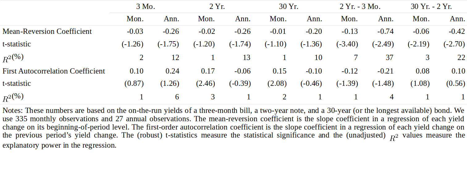
Figure 12 Mean Reversion and Autocorrelation of US Yield Levels and Curve Steepness, 1968-95

Moving to the unexpected part of yield changes, we analyze the behavior of (basis-point) yield volatility over time. In an influential study, Chan, Karolyi, Longstaff, and Sanders (1992) show that various specifications of common one-factor term structure models differ in two respects: the degree of mean reversion and the level-dependency of yield volatility. Empirically, they find insignificant mean reversion and significantly level-dependent volatility —— more than a one-for one relation.^[16] Moreover, they find that the evaluation of various one-factor models' realism depends crucially on the volatility assumption; models that best fit US data have a level-sensitivity coefficient of 1.5. According to these models, future yield volatility depends on the current rate level and nothing else: High yields predict high volatility. Another class of models —— so called GARCH models —— stipulate that future yield volatility depends on the past volatility: High recent volatility and large recent shocks (squared yield changes) predict high volatility. Brenner, Harjes and Kroner (1996) show that empirically the most successful models assume that yield volatility depends on the yield level and on past volatility. With GARCH effects, the level-sensitivity coefficient drops to approximately 0.5. Finally, all of these studies include the exceptional period 1979-82 which dominates the results (see Figure 13). In this period, yields rose to unprecedented levels —— but the increase in yield volatility was even more extraordinary. Since 1983, the US yield volatility has varied much less closely with the rate level.^[17]

转移到收益率变化的非预期部分，我们分析（基点）收益率波动率随时间的变化行为。Chan，Karolyi，Longstaff 和 Sanders（1992）在一个有影响力的研究中表明，常见的单因子期限结构模型在两个方面有所不同：均值回归的程度和波动率对收益率水平的依赖。经验上，他们发现均值回归是微不足道的而波动率显著依赖收益率水平。此外，他们发现，评估各种单因子模型在很大程度上取决于波动性假设，最适合美国数据的模型收益率水平敏感系数为1.5。根据这些模型，未来收益率波动率仅仅取决于当前的收益率水平，所以，高收益率预示高波动率。另一类模型，即所谓的 GARCH 模型，规定未来收益率波动率取决于过去的波动率：近期波动率较大和近期的大幅震荡（平均收益率变化）预示高波动率。Brenner，Harjes 和 Kroner（1996）表明，经验上最成功的模型假设收益率波动率取决于收益率水平和过去的波动率。考虑到 GARCH 效应，收益率水平敏感度系数降至约0.5。最后，所有这些研究都包括了1979-82年这一特殊时期，并主导着结果（见图13）。在这一时期，收益率上升到前所未有的水平，收益率波动率的增加更是巨大。自1983年以来，美国的收益率波动率与收益率水平关系不大。

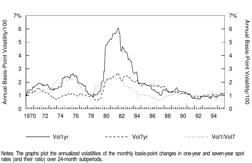
Figure 13 24-Month Rolling Spot Rate Volatilities in the United States

A few words about the required bond risk premia. In all one-factor models, the bond risk premium is a product of the market price of risk, which is assumed to be constant, and the amount of risk in a bond. Risk is proportional to return volatility, roughly a product of duration and yield volatility. Thus, models that assume rate-level-dependent yield volatility imply that the bond risk premia vary directly with the yield level. Empirical evidence indicates that the bond risk premia are not constant —— but they also do not vary closely with either the yield level or yield volatility (see Figure 2 in Part 4). Instead, the market price of risk appears to vary with economic conditions, as discussed above Figure 4. One point upon which theory and empirical evidence agree is the sign of the market price of risk. Our finding that the bond risk premia increase with return volatility is consistent with a negative market price of interest rate risk. (Negative market price of risk and negative bond price sensitivity to interest rate changes together produce positive bond risk premia.) Many theoretical models, including the Cox-Ingersoll-Ross model, imply that the market price of interest rate risk is negative as long as changing interest rates covary negatively with the changing market wealth level.

关于债券风险溢价要说几句话。在所有单因子模型中，债券风险溢价是风险市场价格（假定为不变）和债券风险量的乘积。风险与回报波动率成正比，大致是久期和收益率波动率的乘积。因此，假设收益率水平依赖的收益率波动率模型意味着债券风险溢价与收益率水平直接相关。经验证据表明，债券风险溢价不是恒定的，但它们也不会随收益率水平或收益率波动率而变化（见第4部分，图2）。相反，风险的市场价格似乎随着经济状况而变化，如上图4所述。理论和实证证据一致的一点是风险市场价格的符号。我们发现，债券风险溢价随回报波动率的增加而与负的收益率风险市场价格一致（负的风险市场价格和负的债券价格对收益率变动的敏感性共同产生正的债券风险溢价）。许多理论模型，包括 Cox-Ingersoll-Ross 模型，都认为收益率风险的市场价格为负，只要收益率随着市场财富水平的变化而反向变化。

Cross-Sectional Evidence

横截面证据

We first discuss the shape of the term structure of yield volatilities and its implications for bond risk measures and later describe the correlations across various parts of the yield curve. The term structure of basis-point yield volatilities in Figure 14 is steeply inverted when we use a long historical sample period. Theoretical models suggest that the inversion in the volatility structure is mainly due to mean-reverting rate expectations (see Appendix A). Intuitively, if long rates are perceived as averages of expected future short rates, temporary fluctuations in the short rates would have a lesser impact on the long rates. The observation that the term structure of volatility inverts quite slowly is consistent with expectations for very slow mean reversion. In fact, after the 1979-82 period, the term structure of volatility has been reasonably flat —— as evidenced by the ratio of short rate volatility to long rate volatility in Figure 13. The subperiod evidence in Figure 14 confirms that the term structure of volatility has recently been humped rather than inverted. The upward slope at the front end of the volatility structure may reflect the Fed's smoothing (anchoring) of very short rates while the one- to three-year rates vary more freely with the market's rate expectations and with the changing bond risk premia.

我们首先讨论收益率波动率的期限结构形状及其对债券风险度量的影响，并且稍后描述收益率曲线的各个部分之间的相关性。当我们使用漫长的历史样本周期时，图14中基点收益率波动率的期限结构迅速倒挂。理论模型表明，波动率结构的倒挂主要是由于均值回归的收益率预期（见附录A）。直观地说，如果长期收益率被视为预期未来短期收益率的平均水平，短期收益率的暂时波动对长期收益率的影响较小。波动性期限结构相当缓慢倒挂的观察结果与非常缓慢的均值回归的预期一致。实际上在1979-82年期间之后，波动率的期限结构相当平坦，这由图13所示的短期波动率与长期波动率的比率证明。图14中的子样本证据证实了波动率的期限结构最近已经不倒挂了。波动率结构前端的向上倾斜可能反映了美联储对非常短期的收益率的平滑（固定），而一年到三年的收益率更为自由地随市场收益率预期和债券风险溢价的变化而变化。

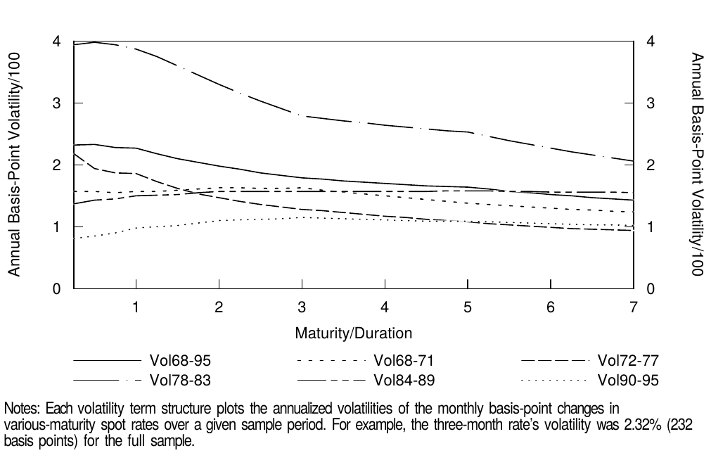
Figure 14 Term Structure of Spot Rate Volatilities in the United States

The nonflat shape of the term structure of yield volatility has important implications on the relative riskiness of various bond positions. The traditional duration is an appropriate risk measure only if the yield volatility structure is flat. We pointed out earlier that inverted or humped yield volatility structures would make the return volatility curve a concave function of duration. Figure 15 shows examples of flat, humped and inverted yield volatility structures (upper panel) —— and the corresponding return volatility structures (lower panel). The humped volatility structure reflects empirical yield volatilities in the 1990s, while the flat and inverted volatility structures are based on the Vasicek model with mean reversion coefficients of 0.00, 0.05, and 0.10. The model's short-rate volatility is calibrated to match that of the three-month rate in the 1990s (77 basis points or 0.77%). It is clear from this figure that the traditional duration exaggerates the relative riskiness of long bonds whenever the term structure of yield volatility is inverted or humped. Moreover, the relative riskiness will be quite misleading if the assumed volatility structure is inverted (as in the long sample period in Figure 14) while the actual volatility structure is flat or humped (as in the 1990s).

收益率波动率期限结构的非平坦形状对各种债券头寸的相对风险具有重要意义。只有当收益率波动率结构平坦时，传统的久期才是适当的风险度量。我们以前指出，倒挂或隆起的收益率波动率结构将使回报波动率曲线成为久期的上凸函数。图15示出了平坦、隆起和倒挂的收益率波动率结构（上图）和相应的回报波动率结构（下图）的实例。隆起的波动率结构反映了1990年代的经验收益率波动率，而平坦和倒挂的波动率结构基于 Vasicek 模型，均值回归系数分别为0.00，0.05和0.10。该模型的短期波动率被校准为与1990年代的三月期收益率（77个基点或0.77%）相一致。从这个数字可以看出，只要收益率波动率的期限结构倒挂或隆起，传统的久期就会夸大长期债券的相对风险。此外，相对风险将会误导投资者，如果假设的波动率结构倒挂（如图14中的长期样本期间），而实际波动率结构平坦或隆起（如1990年代）。

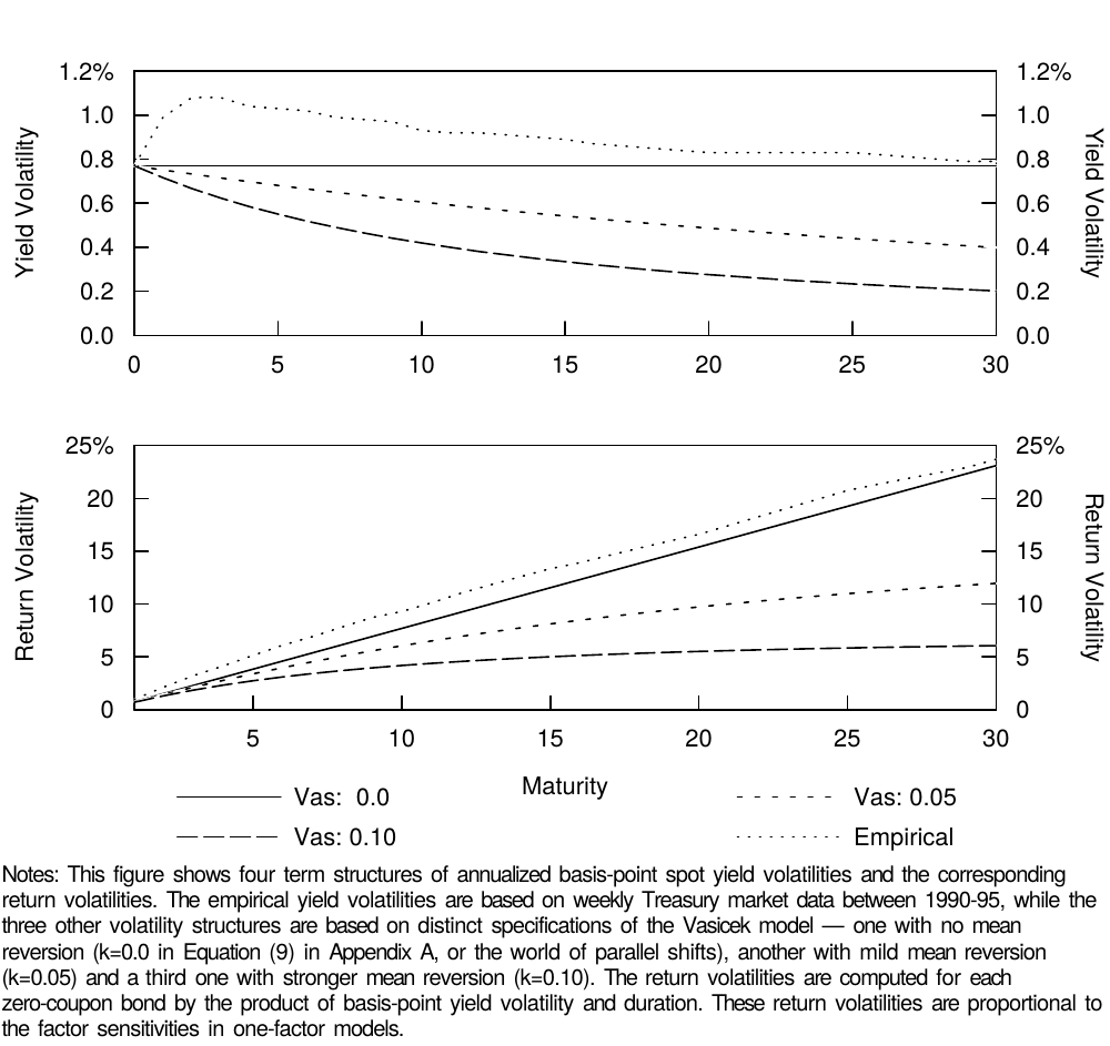
Figure 15 Basis-Point Yield Volatilities and Return Volatilities for Various Models

Historical analysis shows that correlations of yield changes across the Treasury yield curve are not perfect but are typically very high beyond the money market sector (0.82-0.98 for the monthly changes of the two, to 30-year on-the-run bonds between 1968-95) and reasonably high even for the most distant points, the three-month bills and 30-year bonds (0.57). Thus, the evidence is not consistent with a one-factor model, but it appears that two or three systematic factors can explain 95%-99% of the fluctuations in the yield curve (see Garbade (1986), Litterman and Scheinkman (1991), Ilmanen (1992)). Based on the patterns of sensitivities to each factor across bonds of different maturities, the three most important factors are often interpreted as the level, slope and curvature factors.^[18]

历史分析显示，国债收益率曲线上收益率变化的相关性不是完全的，但通常非常高于货币市场（1968之1995年之间，2到30年期债券收益率的月度相关性为0.82-0.98），即使是期限间隔最远的两点，三月期国库券和三十年期债券收益率的相关性也是相当高的（0.57）。因此，证据与单因子模型不一致，但似乎两个或三个系统因子可以解释收益率曲线的95%-99%波动（参见 Garbade（1986），Litterman 和 Scheinkman（1991），Ilmanen（1992））。根据不同期限债券对每个因子的敏感度模式，三个最重要的因子通常被解释为水平、斜率和曲率因子。

APPENDIX A. A SURVEY OF TERM STRUCTURE MODELS^[19]

期限结构综述

A vast literature exists on quantitative modeling of the term structure of interest rates. Because of the large number of these models and the fact that the use of stochastic calculus is needed to derive these models, many investors view them as inaccessible and not useful for their day-to-day portfolio management. However, investors use these models extensively in the pricing and hedging of fixed-income derivative instruments and, implicitly, when they consider such measures as option-adjusted spreads or the delivery option in Treasury bond futures. Furthermore, these models can provide useful insights into the relationships between the expected returns of bonds of different maturities and their time-series properties. It is important that investors understand the assumptions and implications of these models to choose the appropriate model for the particular objective at hand (such as valuation, hedging or forecasting) and that the features of the chosen model are consistent with the investor's beliefs about the market. Although the models are developed through the use of stochastic calculus, it is not necessary that the investor have a complete understanding of these techniques to derive some insight from the models. One goal of this section is to make these models accessible to the fixed-income investor by relating them to risk concepts with which he is familiar, such as duration, convexity and volatility.

关于收益率期限结构的量化模型已经出现了大量文献。由于这些模型数量众多，而且需要使用随机分析来推导这些模型，许多投资者认为它们是无法理解的，对于他们的日常投资组合管理毫无用处。然而，投资者在固定收益衍生品的定价和对冲中广泛使用这些模型，并且在考虑期权调整利差或国债期货交割期权等度量是也隐含地使用这些模型。此外，这些模型可以为不同期限债券的预期回报与其时间序列特征之间的关系提供有用的见解。投资者必须了解这些模型的假设和影响，以为特定用途（例如估值、对冲或预测）选择适当的模型，并且所选模型的特征要与投资者对市场的信念相一致。虽然这些模型通过使用随机分析构造出来，但投资者并不需要先对这些技术有完全的了解再从模型中得出一些见解。本节的一个目标是使固定收益投资者可以将这些模型与他熟悉的风险概念相关联，例如久期、凸度和波动率。

Equation (1) in Part 5 of this series gives the expression of the percentage change in a bond's price (\(\Delta P/P\)) as a function of changes in its own yield (\(\Delta y\)).

本系列第5部分中的方程式（1）给出了债券价格变动百分比（\(\Delta P/P\)）作为自身收益率变化（\(\Delta y\)）函数的表达式。

\[100 * \Delta P/P \approx -Duration * \Delta y + 0.5 * Convexity * (\Delta y)^2. \tag{1} \]

This expression, which is derived from the Taylor series expansion of the price-yield formula, is a perfectly valid linkage of changes in a bond's own yield to returns and expected returns through traditional bond risk measures such as duration and convexity.

这一表达式从价格-到期收益率公式的泰勒级数展开得到，将债券自身到期收益率变化与回报和预期回报通过传统的债券风险度量（如久期和凸度）完美的联系起来。

One problem with this approach is that every bond's return is expressed as a function of its own yield. This expression says nothing about the relationship between the return of a particular bond and the returns of other bonds. Therefore, it may have limited usefulness for hedging and relative valuation purposes. One must impose some simplifying assumptions to make these equations valid for cross-sectional comparisons. In particular, more specific assumptions are needed for the valuation of derivative instruments and uncertain cash flows. Of course, the marginal value of more sophisticated term structure models depends on the empirical accuracy of their specification and calibration.

这种方法的一个问题是每个债券的回报都表示为其自身到期收益率的函数。这种表示不涉及特定债券回报与其他债券回报之间的关系。因此，对于对冲和衡量相对价值来说用途可能有限。必须强加一些简化的假设，使这些方程对于横向比较是有效的。特别是，对衍生品的估值和不确定的现金流需要更具体的假设。当然，更复杂的期限结构模型的边际价值取决于其具体形式和校准的经验准确性。

Factor Model Approach

因子模型方法

Term structure models typically start with a simple assumption that the prices of all bonds can be expressed as a function of time and a small number of factors. For ease of explanation, the analysis is often restricted to default-free bonds and their derivatives. We first discuss one-factor models which assume that one factor (\(F_t\))^[20] drives the changes in all bond prices and the dynamics of the factor is given by the following stochastic differential equation:

期限结构模型通常从简单的假设开始，即所有债券的价格可以表达为时间和少数因子的函数。为了便于解释，分析往往限于无违约债券及其衍生品。我们首先讨论单因子模型，假设一个因子（\(F_t\)）驱动所有债券价格的变化，因子的动态变化由以下随机微分方程给出：

\[\frac{dF}{F} = m(F,t)dt + s(F,t)dz \tag{2} \]

where F can be any stochastic factor such as the yield on a particular bond or the real growth rate of an economy, dt is the passage of a small (instantaneous) time interval, and dz is Brownian motion (a random process that is normally distributed with a mean of 0 and a standard deviation of \(\sqrt{dt}\)). The letter "d" in front of a variable can be viewed as shorthand for "change in". Equation (2) is an expression for the percentage change of the factor which is split into expected and unexpected parts. The "drift" term \(m(F,t)dt\) is the expected percentage change in the factor (over a very short interval dt). This expectation can change as the factor level changes or as time passes. In the unexpected part, \(s(F,t)\) is the volatility of the factor (also dependent on the factor level and on time) and dz is Brownian motion. For now, we leave the expression of the factors as general, but various one-factor models differ by the specifications of \(m(F,t)\) and \(s(F,t)\).

其中 F 可以是任何随机因子，如一个特定债券的收益率或一个经济体的实际增长率，dt 是一个小的（瞬时的）时间间隔，dz 是布朗运动（一个服从正态分布的随机过程，平均值为0，标准偏差为\(\sqrt{dt}\)）。变量前面的字母“d”可以被视为“变化”的缩写。方程（2）将因子百分比变化分解为预期和非预期部分。“漂移”项\(m(F,t)dt\)是因子的预期百分比变化（在非常短的时间间隔dt内）。这个预期可以随着因子水平或时间的变化而改变。在非预期部分，\(s(F,t)\)是因子的波动率（也取决于因子水平和时间），dz是布朗运动。现在，我们将这些因子的表达式一般化，各种单因子模型根据\(m(F,t)\)和\(s(F,t)\)的具体形式而有所不同。

Let the price at time t of a zero-coupon bond which pays $1 at time T be expressed as \(P_i(F,t,T)\). Because F is the only stochastic component of \(P_i\), Ito's Lemma —— roughly, the stochastic calculus equivalent of taking a derivative —— gives the following expression for the dynamics of the bond price:

假定在时间 T 支付$1的零息债券在时间 t 的价格表示为\(P_i(F,t,T)\)。因为 F 是\(P_i\)的唯一随机成分，所以根据 Ito 引理——大致相当于定义在随机分析上的导数，给出了以下债券价格动态的表达式。

\[\frac{dP_i(F,t,T)}{P_i} = \mu_i dt + \sigma_i dz \tag{3} \]

where \(\mu_i = \frac{\partial P_i}{\partial t} \frac{1}{P_i} + \frac{\partial P_i}{\partial F} \frac{1}{P_i} m(F,t)F + \frac{1}{2} \frac{\partial^2 P_i}{\partial F^2} \frac{1}{P_i} s(F,t)^2F^2\), and \(\sigma_i = \frac{\partial P_i}{\partial t} \frac{1}{P_i} s(F,t)F\).

其中\(\mu_i = \frac{\partial P_i}{\partial t} \frac{1}{P_i} + \frac{\partial P_i}{\partial F} \frac{1}{P_i} m(F,t)F + \frac{1}{2} \frac{\partial^2 P_i}{\partial F^2} \frac{1}{P_i} s(F,t)^2F^2\)，并且\(\sigma_i = \frac{\partial P_i}{\partial t} \frac{1}{P_i} s(F,t)F\)。

In this framework, Ito's Lemma gives us an expression for the percentage change in price of the bond over the time dt for a given realization of F at time t. \(\mu_i\) is the expected percentage change in the price (drift) of bond i over the period dt and \(\sigma_i\) is the volatility of bond i.

在这个框架下，Ito引理给出了 t 时刻给定实现的 F 情况下债券价格变化百分比的表达式。\(\mu_i\)是债券 i 在时间 dt 内的价格预期百分比变化（漂移），\(\sigma_i\)是债券 i 的波动率。

The unexpected part of the bond return depends on the bond's "duration" with respect to the factor (its factor sensitivity)^[21] and the unexpected factor realization. The return volatility of bond i (\(\sigma_i\)) is the product of its factor sensitivity and the volatility of the factor.

债券回报的非预期部分取决于债券的“久期”关于因子（因子敏感度）和非预期因子的实现。债券 i 的回报波动率（\(\sigma_i\)）是其因子敏感度和因子波动率的乘积。

Equation (3) shows that the decomposition of expected returns in Part 6 of this series is very general. The expected part of the bond return over dt is given by the expected percentage price change \(\mu_i\) because zero-coupon bonds do not earn coupon income. Consider the three components of the expected return. (1) The first term is the change in price due to the passage of time. Because our bonds are zero-coupon bonds, this change (accretion) will always be positive and represents a "rolling yield" component; (2) The second term is the expected change in the factor (mF) multiplied by the sensitivity of the bond's price to changes in the factor. This price sensitivity is like "duration" with respect to the relevant factor; and (3) The third term comprises of the second derivative of the price with respect to changes in the factor and the variance of the factor. The second derivative is like "convexity" with respect to the factor.

方程（3）表明本系列第6部分预期回报的分解非常一般化。因为零息债券不会获得票息收入，债券收益率的预期部分由 dt 时间内的预期价格变动百分比\(\mu_i\)给出。考虑预期回报的三个组成部分。（1）第一项是由于时间的推移而导致的价格变动。因为我们的债券是零息债券，所以这种变化（增值）将永远是正的，代表着“滚动收益率”的部分；（2）第二项是因子（mF）的预期变化乘以债券价格对因子变化的敏感度。这个价格敏感度相当于相关因子的“久期”；和（3）第三项包括关于因子变化和因子方差的价格二次导数。二次导数相当于因子的“凸度”。

Suppose we specify the factor F to be the yield on bond i (\(y_i\)). Then, the expected change in price of bond i over the short time period (dt) is given by the familiar equation that we developed in the previous parts of this series:

假设我们将因子 F 指定为债券 i 的收益率（\(y_i\)）。那么，短期内（dt）债券 i 的价格预期变化是由本系列前面部分所得到的方程给出的：

\[\begin{aligned} E\left(\frac{dP_i(y,t,T)}{P_i} \right) &= \mu_i dt = \frac{\partial P_i}{\partial t} \frac{1}{P_i} + \frac{\partial P_i}{\partial y_i} \frac{1}{P_i}E(\Delta y_i) + \frac{1}{2}\frac{\partial^2 P_i}{\partial y_i^2} \frac{1}{P_i} variance(\Delta y_i)\\ &= \textit{Rolling Yield}_i - Duration_i*E(\Delta y_i) + \frac{1}{2}Convexity_i*variance(\Delta y_i) \end{aligned} \tag{4} \]

where \(\Delta y_i\) is the change in the yield of bond i. We can also use Equation (4) to similarly link the factor model approach to the decompositions of forward rates made in the previous parts of this series. It can be shown (for "time-homogeneous" models) that the instantaneous forward rate T periods ahead equals the rolling yield component. Therefore, we rewrite Equation (4) in terms of the forward rate as follows:

其中\(\Delta y_i\)是债券 i 收益率的变化。我们也可以使用等式（4）将因子模型方法与本系列前面部分中的远期收益率分解类比。可以显示（对于“时齐”模型），即T年期瞬时远期收益率等于滚动收益率分量。因此，我们根据远期收益率重写等式（4）如下。

\[\begin{aligned} f_{T, T+dt} &= \frac{\partial P_i}{\partial t} \frac{1}{P_i} = E\left(\frac{dP_i}{P_i} \right) - \frac{\partial P_i}{\partial y_i} \frac{1}{P_i}E(\Delta y_i) - \frac{1}{2}\frac{\partial^2 P_i}{\partial y^2_i} \frac{1}{P_i} variance(\Delta y_i) \\ &= \textit{Expected Yield}_i + Duration_i*E(\Delta y_i) - \frac{1}{2}Convexity_i*variance(\Delta y_i) \end{aligned} \tag{5} \]

The expected return term can be further decomposed into the risk-free short rate and the risk premium for bond i. Thus, forward rates can be decomposed into the rate expectation term (drift), a risk premium term and a convexity bias (or a Jensen's inequality) term. Other term structure models contain analogous but more complex terms.

预期回报项可以进一步分解为无风险短期收益率和债券 i 的风险溢价。因此，远期收益率可以分解为收益率预期（漂移）、风险溢价和凸度偏差（或Jensen不等式）。其他期限结构模型包含类似但更复杂的成分。

Unfortunately, by defining the one relevant factor to be the bond's own yield, Equation (4) only holds for bond i. For any other bond j, the chain rule in calculus tells us that

不幸的是，因为将一个相关因子限定在债券自身收益率上，方程（4）仅适用于债券 i。对于任何其他债券 j，结论中的链式规则告诉我们

\[-\frac{\partial P_i}{\partial y_i} \frac{1}{P_i} = \frac{\partial P_i}{\partial y_j} \frac{\partial y_j}{\partial y_i} \frac{1}{P_i} \text{ which equals } Duration_j \text{ only if } \frac{\partial y_j}{\partial y_i} = 1 \tag{6} \]

Therefore, in a one-factor world where \(y_i\) represents the relevant factor, Equation (4) only holds for bonds other than bond i if all shifts of the yield curve are parallel. While this observation suggests that more sophisticated term structure models are needed for derivatives valuation, it does not deem useless the framework developed in this series. In particular, this framework is valuable in applications such as interpreting yield curve shapes and forecasting the relative performance of various government bond positions. Such forecasts are not restricted to parallel curve shifts if we predict separately each bond's yield change (or if we predict a few points in the curve and interpolate between them). The problem with using maturity-specific yield and volatility forecasts is that the consistency of the forecasts across bonds and the absence of arbitrage opportunities are not explicitly guaranteed.

因此，在单因子世界中\(y_i\)代表相关因子，如果收益率曲线的所有变动是平行的，则式（4）适用于债券 i 以外的债券。虽然这一观察结果表明衍生品估值需要更复杂的期限结构模型，但在本系列中制定的框架并非是无用的。特别地，这个框架在解释收益率曲线形状和预测各种政府债券头寸相对表现的应用中是有价值的。如果我们单独预测每个债券的收益率变化（或者如果我们预测曲线中的几个点并在它们之间插值），那么这种预测并不局限于平行的曲线偏移。使用特定期限收益率和波动率预测的问题是，债券之间预测的一致性和无套利机会没有明确的保证。

Arbitrage-Free Restriction

无套利约束

For the time being, we return to the world where the factor, F, is unspecified and the change in price (return) of any bond i is given by Equation (3). How should bonds be priced relative to each other? The first term of Equation (3) is deterministic —— that is, we know today what the value of this component will be at the end of time t+dt. However, the value of second term is unknown until the end of time t+dt. In fact, in this one-factor framework, this is the only unknown component of any bond's returns. If we can form a portfolio whereby we eliminate all exposure to the one stochastic factor, then the return on the portfolio is known with certainty. If the return is known with certainty, then it must earn the riskless rate r or else arbitrage opportunities would exist.

回到问题上来，其中因子 F 是未指定的，并且任何债券 i 的价格（回报）变化由公式（3）给出。债券如何相对于彼此定价？方程（3）的第一项是确定性的，也就是说，我们今天知道在时间t+dt结束时这个部分的值。然而，第二项的值直到时间t+dt结束是未知的。事实上，在这个单因子框架下，这是任何债券回报中唯一未知的组成部分。如果我们可以构造一个投资组合消除这个随机因素的所有风险，那么投资组合的回报是确定的。如果回报是确定的，那么它必须获得无风险收益率 r ，或者套利机会将会存在。

It also follows that in our one-factor world, the ratio of expected excess return over the return volatility must be equal for any two bonds to prevent arbitrage opportunities. This relation must hold for all bonds or portfolios of bonds, and in Equation (7) below is the value of this ratio, often known as the "market price of the factor risk".

同样，在我们的单因子世界中，为防止套利机会存在，任何两个债券的预期超额回报与回报波动率的比率必须相等。这种关系必须适用于所有债券或债券组合，下面的方程（7）是该比率的价值，通常称为“因子风险的市场价格”。

\[\frac{\mu_1 - r}{\sigma_1} = \frac{\mu_2 - r}{\sigma_2} = \lambda \tag{7} \]

where r is the riskless short rate

其中 r 是无风险短期收益率。

Solutions of the Term Structure Models for Bond Prices

期限结构模型关于债券价格的解

Combining Equations (3) and (7) leads to the following differential equation:

组合方程（3）和（7）得到以下微分方程。

\[\frac{\partial P_1}{\partial t} + \frac{\partial P_1}{\partial F}(mF -\lambda s) + \frac{1}{2} \frac{\partial^2 P_1}{\partial F^2} s^2 F^2 = r P_1 . \tag{8} \]

This differential equation is solved to obtain bond prices and derivatives of bonds. Virtually all of the existing one-factor term-structure models are developed in this framework.^[22] The next step is to impose a set of boundary conditions specific to the instrument that is being priced and then solve the differential equation for \(P(F,t,T)\). One boundary condition for zero-coupon bonds is that the price of the bond at maturity is equal to par (\(P(F,T,T)=100\)). Another example of a boundary condition is that the value of a European call option on bonds, at the expiration of the option, is given by \(C(t,T,K) = \max[P(F,t,T)-K,0]\). Various term structure models differ in the definition of the relevant factor and the specification of its dynamics. Specifically, the one-factor models differ from each other in how the variable F and the functions m(F,t) (factor drift) and s(F,t) (factor volatility) are specified. Different specifications lead to distinct solutions of Equation (8) and distinct implications for bond prices and yields. In the rest of this section, we will analyze one such specification to give the reader an intuitive interpretation of these models, and then we qualitatively discuss the trade-offs between various popular models.

解这个微分方程可以获得债券价格和债券衍生品。几乎所有现有的单因子期限结构模型都是在这个框架下开发的。下一步是对金融产品施加一组特定的边界条件，然后求解\(P(F,t,T)\)的微分方程。零息债券的一个边界条件是债券在到期时的价格等于面值（\(P(F,T,T)=100\)）。边界条件的另一个例子是在期权到期时，债券上的欧式看涨期权的价值由\(C(t,T,K) = \max[P(F,t,T)-K,0]\)给出。各种期限结构模型在相关因子的定义和其动态结构上有所不同。具体来说，单因子模型在如何规定变量 F 和函数m(F,t)（因子漂移）和s(F,t)（因子波动率）之间彼此不同。不同的规定导致方程（8）的不同解，对债券价格和收益率有明显的影响。在本节的其余部分，我们将分析一个规定用来为读者直观地解释这些模型，然后定性地讨论如何在各种流行模型之间权衡。

One Example: The Vasicek Model

示例：Vasicek 模型

Many of the existing term-structure models begin by specifying the one stochastic factor that affects all bond returns as the riskless interest rate (r) on an investment that matures at the end of dt. One of the earliest such model developed by Vasicek (1977) took this approach and specified the dynamics of the short rate as follows:

许多现有的期限结构模型首先指定影响所有债券回报的一个随机因子，作为在 dt 到期的投资的无风险收益率（r）。最早由Vasicek（1977）开发的一个模型采用了这种方法，并指出短期收益率的动态结构如下：

\[dr = k(l-r)dt + s dz. \tag{9} \]

This fits in the framework of Equation (2) if F is defined to be r and \(m(r,t) = (k(l-r))/r\) and \(s(r,t)=s/r\). The second term indicates that the short rate is normally distributed with a constant volatility of s which does not depend on the current level of r. The basis-point yield volatility is the same regardless of whether the short rate is equal to 5% or 20%. The drift term requires some interpretation. In the Vasicek model, the short rate follows a mean-reverting process. This means that there is some long-term mean level toward which the short rate tends to move. If the current short rate is high relative to this long-term level, the expected change in the short-rate is negative. Of course, even if the expected change over the next period is negative, we do not know for sure that the actual change will be negative because of the stochastic component. In Equation (9), l is the long-term level of the short rate and k is the speed of mean-reversion. If k = 0, there is no mean-reversion of the short rate. If k is large, the short rate reverts to its long-term level quite quickly and the stochastic component will be small relative to the mean reversion component.

如果 F 定义为 r，并且\(m(r,t) = (k(l-r))/r\)，\(s(r,t)=s/r\)，则符合等式（2）的框架。第二项表示短期收益率服从正态分布，常波动率 s 不依赖于目前 r 的水平。无论短期收益率是否等于5%或20%，基点收益率波动率是相同的。漂移项需要一些解释。在 Vasicek 模型中，短期收益率遵循均值回归过程。这意味着短期收益率趋向于回到某个长期平均水平。如果目前的短期收益率相对于长期水平较高，短期收益率的预期变动将是负的。当然，即使下一期的预期变化是负的，由于随机因素，我们不知道实际的变化是否将是负的。在等式（9）中，l 是短期收益率的长期水平，k 是均值回归的速度。如果k = 0，则不存在短期收益率的均值回归。如果 k 比较大，则短期收益率会相当快地回复到长期水平，随机部分相对于均值回归部分将比较小。

This specification falls into a class of models known as the "affine" yield class. "Affine" essentially means that all continuously compounded spot rates are linear in the short rate. Many of the popular one-factor models belong to this class. For the affine term structure models, the solution of Equation (8) for zero-coupon bond prices is of the following form:

这种形式属于所谓“仿射”收益率类的一类模型。“仿射”基本上意味着所有连续复利即期收益率在短期内是线性的。许多受欢迎的单因子模型属于这一类。对于仿射期限结构模型，等式（8）对零息债券价格的解如下。

\[P(r,t,T) = e^{A(t,T) - B(t,T)r} \tag{10} \]

Typically, \(A(t,T)\) and \(B(t,T)\) are functions of the various parameters describing the interest rate dynamics such as k, l, s, and \(\lambda\). It is easy to show that the "duration" of the zero-coupon bond with respect to the short rate equals \(B(t,T)\). How does this duration measure differ from our traditional definition of duration with respect to a bond's own yield? For example, in the Vasicek model, the solution for B(t,T) is given by the following:

通常，\(A(r,t,T)\)和\(B(r,t,T)\)是描述收益率动态结构的各种参数（k、l、s 和\(\lambda\)）的函数。很容易显示零息债券相对于短期收益率的“久期”等于\(B(t,T)\)。这个久期衡量标准与传统相对于债券本身收益率的久期有何不同？例如，在 Vasicek 模型中，\(B(t,T)\)的解如下：

\[B(t,T) = \frac{1-e^{-k(T-t)}}{k} . \tag{11} \]

Therefore, the duration measure with respect to changes in the short rate is a function of the speed of mean-reversion parameter, k. As this parameter approaches 0, the duration of a bond with respect to changes in the short rate approaches the traditional duration measure with respect to changes in the bond's own yield. Without mean reversion, the Vasicek model implies parallel yield shifts, and Equation (4) holds. However, as the mean reversion speed gets larger, long bonds' prices are only slightly more sensitive to changes in the short rate than are intermediate bonds' prices because the impact of longer (traditional) duration is partly offset by the decay in yield volatility (see Figure 15). With mean reversion, long rates are less volatile than short rates. In this case, the traditional duration measure would overstate the relative riskiness of long bonds.

因此，关于短期收益率变化的久期度量是均值回归速度参数 k 的函数。随着这个参数接近0，关于短期收益率变化的债券久期接近于传统的相对于债券本身收益率的久期。如果没有均值回归，Vasicek 模型意味着平行的收益率变化，等式（4）成立。然而，随着均值回归速度变得越来越大，长期债券价格对短期收益率的变化比中期债券价格稍微更敏感，因为（传统的）长久期的影响被收益率波动率的衰退部分抵消了（见图15）。因为均值回归，长期收益率波动率低于短期收益率。在这种情况下，传统的久期度量会夸大长期债券的相对风险。

Comparisons of Various Models

不同模型的比较

Most of the one-factor term structure models that have evolved over the past 20 years are remarkably similar in the sense that they all essentially were derived in the framework that we described above. However, dissatisfaction with certain aspects of the existing technologies have motivated researchers in the industry and in academia to continue to develop new versions of term structure models. Four issues that have motivated the model-builders are:

• Consistency of factor dynamics with empirical observations;
• Ability to fit the current term structure and volatility structure;
• Computational efficiency; and
• Adequacy of one factor to satisfactorily describe the term structure dynamics.

在过去20年中大多数的单因子期限结构模型显然是相似的，因为它们基本都上在我们上面描述的框架中得出的。然而，对现有技术某些方面的不满，促使行业和学术界的研究人员继续开发新版本的期限结构模型。促成模型建立的四个问题是：

• 因子动态结构与经验观察的一致性；
• 拟合当前期限结构和波动率结构的能力；
• 计算效率；以及
• 单因子模型完善地描述期限结构动态的妥当性。

Differing Factor Specifications. Some of the one-factor models differ by the definition of the one common factor. However, the vast majority of the models assume that the factor is the short rate and the models differ by the specification of the dynamics of the factor.

改变因子的形式。一个单因子模型因一个共同因子的定义而有所不同。然而，绝大多数模型都认为这个因子是短期收益率，而且这些模型因这个因子的动态结构而异。

For example, the mean-reverting normally distributed process for the short rate that is used to derive the Vasicek model (Equation (9)) leads to features that many users find problematic. Specifically, nominal interest rates can become negative and the basis-point volatility of the short rate is not affected by the current level of interest rates. The Cox-Ingersoll-Ross model (CIR) is based on the following specification of the short rate which precludes negative interest rates and allows for level-dependent volatility:

例如，用于推导 Vasicek 模型（等式（9））的短期收益率的均值回归正态分布过程导致许多用户发现一个问题。具体来说，名义收益率可能变为负数，并且短期收益率的基点波动率不受当前收益率水平的影响。Cox-Ingersoll-Ross 模型（CIR）基于以下短期收益率的形式，排除了负收益率，并允许依赖收益率水平的波动率。

\[dr = k(l-r)dt + s\sqrt{r} dz . \tag{12} \]

Because this model is a member of the affine yield class, the solution of the model is of the form shown in Equation (10). The function \(B(t,T)\), which represents the "duration" of the zero-coupon bond price with respect to changes in the short rate, is a complex function of the parameters k, l, s, and \(\lambda\). As in the Vasicek model, when the mean-reversion parameter is non-zero, the durations of long bonds with respect to changes in the short rate are significantly lower than the traditional duration.

因为这个模型是仿射收益率类的一个成员，所以模型的解是由式（10）所示。函数\(B(t,T)\)（表示零息债券价格相对于短期收益率变化的“久期”）是参数 k、l、s 和\(\lambda\)的复杂函数。与 Vasicek 模型一样，当均值回归参数为非零值时，长期债券相对于短期收益率变化的久期显着低于传统久期。

Chan, Karolyi, Longstaff and Sanders (CKLS, 1992) empirically compare the various models by noting that most of the one-factor models developed in the 1970s and 1980s are quite similar in that they define the one factor to be the short rate, r, and their dynamics are described by the following equation:

Chan，Karolyi，Longstaff 和 Sanders（CKLS，1992）经验性地比较了各种模型，注意到在1970年代和80年代开发的大多数单因子模型是非常相似的，因为它们将单因子定义为短期收益率，并且它们的动态结构由以下等式描述：

\[dr = k(l-r)dt + s r^\gamma dz . \tag{13} \]

The differences between the models are in their specification of k and \(\gamma\). For example, the Vasicek model has a non-zero k and \(\gamma = 0\). CIR also has a non-zero k and \(\gamma = 0.5\). We discuss the findings of CKLS and subsequent researchers in the section "How Does the Yield Curve Evolve Over Time?".

模型之间的差异在于 k 和\(\gamma\)的形式。例如，Vasicek 模型具有非零 k，且 \(\gamma = 0\)。CIR 模型也具有非零 k，且\(\gamma = 0.5\)。我们在“收益率曲线如何随时间变化”一节中讨论了 CKLS 模型和研究人员的后续发现。

Fitting the Current Yield Curve and Volatility Structure. One of the problems that practitioners have with the early term structure models such as the original Vasicek and CIR models is that the parameters of the short-rate dynamics (k, l, s) and the market price of risk, \(\lambda\), must be estimated using historical data or by minimizing the pricing errors of the current universe of bonds. Nothing ensures that the market prices of a set of benchmark bonds matches the model prices. Therefore, a user of the model must conclude that either the benchmarks are "rich" or "cheap" or that the model is misspecified. Practitioners who must price derivatives from the model typically are not comfortable assuming that the market prices the benchmark Treasury bonds incorrectly.

拟合当前收益率曲线和波动率结构。从业者在使用早期结构模型（如原始的 Vasicek 和 CIR 模型）中发现的一个问题是，必须通过使用历史数据或最小化当前债券的定价错误来估计短期收益率动态因子（k，l，s）和风险市场价格\(\lambda\)。没有什么可以确保一组基准债券的市场价格与模型价格相一致。因此，模型的用户必须得出结论，即基准是“高估的”或“低估的”，或者模型是错误的。假设市场对基准国债的估价不正确，那么用模型进行衍生品定价的从业者通常会感到担忧。

In 1986, Ho and Lee introduced a model that addressed this concern by specifying that the "risk-neutral" drift of the spot rate is a function of time. This addition allows the user to calibrate the model in such a way that a set of benchmark bonds are correctly priced without making assumptions regarding the market price of risk. Subsequently developed models address some shortcomings in the process implied by the Ho-Lee model (possibility of negative interest rates) or fit more market information (term structure of implied volatilities). Such models include Black-Derman-Toy, Black-Karasinski, Hull-White, and Heath-Jarrow-Morton. These models have become known as the "arbitrage-free" models, as opposed to the earlier "equilibrium" models. Our brief discussion does not do justice to these models; interested readers are referred to surveys by Ho (1994) and Duffie (1995).

1986年，Ho 和 Lee 介绍了一个解决这一担忧的模型，指出即期收益率的“风险中性”漂移是时间的函数。添加的这个条件允许用户校准模型，使得一组基准债券的价格是正确的，而不对风险的市场价格做出假设。随后的模型解决了 Ho-Lee 模型所隐含的随机过程出现的一些缺陷（负收益率的可能性），或者使模型可以适应更多的市场信息（隐含波动率的期限结构）。这些模型包括 Black-Derman-Toy、Black-Karasinski、Hull-White 和 Heath-Jarrow-Morton 模型。这些模型被称为“无套利”模型，而不是早期的“均衡”模型。我们的简短讨论不对这些模型评判，有兴趣的读者请参考 Ho（1994）和 Duffie（1995）的综述。

These arbitrage-free models represent the current "state of the art" for pricing and hedging fixed-income derivative instruments. One theoretical problem with these models is that they are time-inconsistent. The models are calibrated to fit the market data and then bonds and derivatives are priced with the implicit assumption that the parameters of the stochastic process remain as specified. However, as soon as the market changes, the model needs to be recalibrated, thereby violating the implicit assumption (see Dybvig (1995)). In reality, most practitioners find this inconsistency a small price to pay for the ability to calibrate the model to market prices.

这些无套利模型代表了当前固定收益衍生品定价和对冲中的“发展水平”。这些模型的一个理论问题是它们是时间不一致的。模型被校准以适应市场数据，然后债券和衍生品的定价隐含地假定随机过程的参数保持当前水平。然而，一旦市场发生变化，模型就需要重新校准，从而违反了隐含的假设（参见Dybvig（1995））。实际上，大多数从业者发现这种不一致性是为了将模型校准到市场价格而付出的代价。

Computational Efficiency. Some of the issues in choosing a model involve computational efficiency. For example, some of the models have the feature that the price of bonds and many derivatives on bonds have a closed-form solution, but others must be solved numerically by techniques such as Monte Carlo methods and finite differences. Because such techniques can be employed quite quickly, most practitioners do not feel that a closed-form solution is necessary. However, a closed-form solution allows a better understanding of the model and the sensitivities of the price to the various input variables.

计算效率。选择模型涉及一些计算效率上的问题。例如，一些模型保证债券价格和债券上的衍生品具有闭式解，而其他模型必须通过诸如蒙特卡罗方法和有限差分之类的技术进行数值求解。因为这样的技术可以很快地执行，所以大多数从业者并不觉得需要一个闭式解。然而，闭式解可以更好地了解模型和价格对各种输入变量的敏感度。

Many practitioners and researchers prefer the Heath-Jarrow-Morton model, which specifies the entire term structure as the underlying factor, because it provides the user with the most degrees of freedom in calibrating the model. However, the major shortcoming of this model is that, when implemented on a lattice (or tree) structure, the nodes of the lattice do not recombine. Therefore, the number of nodes grows exponentially as the number of time steps increase, rendering the time to obtain a price unacceptably long for many applications. Much of the recent research has been devoted to approximating this model to make it more computationally efficient.

许多从业者和研究人员喜欢使用 Heath-Jarrow-Morton 模型（它将整个期限结构指定为潜在因子），因为它为用户校准模型提供最大的自由度。然而，该模型的主要缺点是，当在网格（或树）结构上实现时，网格的节点不会重合。因此，随着时间步长的增加，节点的数量呈指数增长，使得许多应用程序具有不可接受的过长计算时间。最近的许多研究已经致力于近似该模型，使其计算效率更高。

Extensions to Multi-Factor Models. Empirical analysis by Litterman and Scheinkman (1991), among others, shows that two or three factors can explain most of the cross-sectional differences in Treasury bond returns. A glance at the imperfect correlations between bond returns provides even simpler evidence of the insufficiency of a one-factor model. Yet, while multi-factor models, by definition, explain more of the dynamics of the term structure than a one-factor model, the cost of the additional complexity and computational time can be significant. In assessing whether a one-, two- or three-factor model is appropriate, the tradeoff is the efficiency gained in pricing and hedging because of the additional factors against these costs. For certain applications in the fixed-income markets, a one-factor model is adequate. For a systematic and detailed comparison of one-factor models vs two-factor models, see Canabarro (1995).

扩展到多因子模型。Litterman 和 Scheinkman（1991）的实证分析显示，两个或三个因素可以解释国债回报的大部分横截面差异。债券回报之间不完全的相关性，提供了揭示单因子模型不足的简单证据。然而，虽然根据定义多因子模型比单因子模型解释了更多的期限结构的动态特征，但是额外的复杂性和计算时间的成本可能是显着的。在评估一、二或三因子模型是否合适时，需要权衡由于添加因子带来的成本与获得的定价和对冲效率。对于固定收益市场的某些应用，单因子模型是足够的。对于单因子模型与双因子模型的系统详细比较，参见 Canabarro（1995）。

The general framework in which a multi-factor term structure model is derived is similar to the one-factor model with the n factors specified in a similar manner as in Equation (2):

导出多因子期限结构模型的一般性框架类似于通过类似等式（2）的方式指定 n 个因子的单因子模型。

\[\frac{dF_j}{F_j} = m_j(F_j, t)dt + s_j(F_j, t) dz_j . \tag{14} \]

where \(j = 1, \dots , n\) and the \(dz_j\)'s can be correlated with correlations given by \(\rho _{jk}(F,t)\).

其中\(j = 1, \dots , n\)，并且\(dz_j\)之间的相关性通过\(\rho _{jk}(F,t)\)给出。

For example, the Cox-Ingersoll-Ross model can be extended into a multi-factor model. To keep the analysis tractable, most term structure models define a small number of factors (n = 2 or 3). Some examples in the literature include the Brennan-Schwartz model, which specifies the two factors as a long and a short rate, the Brown-Schaefer model, which specifies the two factors as a long rate and the yield curve steepness, the Longstaff-Schwartz model, which specifies the two factors as a short rate and the volatility of the short rate, and the Duffie-Kan model, which specifies the factors as the yields on n bonds. A multi-factor version of Ito's Lemma provides the following expression for the return of bonds in the multi-factor world:

例如，Cox-Ingersoll-Ross 模型可以扩展到多因子模型。为了使分析易于处理，大多数期限结构模型定义了少量因子（n = 2或3）。文献中的一些例子包括 Brennan-Schwartz 模型，将其两个因子指定为长期和短期收益率，Brown-Schaefer 模型，将起两个因子指定为长期收益率和收益率曲线陡峭程度，Longstaff-Schwartz 模型，将其两个因子指定为短期收益率和短期收益率的波动率，以及 Duffie-Kan 模型，将其因子指定为 n 个债券的收益率。Ito引理的多因子版本为多因子世界中债券的回报提供了以下表达式：

\[\frac{dP_i(F,t,T)}{P_i} = \mu_i dt + \sigma_i dz , \tag{15} \]

where \(\mu_i = \frac{\partial P_i}{\partial t} \frac{1}{P_i} + \sum_{j=1}^n \frac{\partial P_i}{\partial F_j} \frac{1}{P_i} m_j(F,t)F_j + \frac{1}{2}\sum_{j=1}^n \sum_{k=1}^n \frac{\partial^2 P_i}{\partial F_j \partial F_k} \frac{1}{P_i} s_j(F,t) s_k(F,t) \rho_{jk}(F,t)F_jF_k\) and \(\sigma_i = \sum_{j=1}^n \frac{\partial P_i}{\partial F_j} \frac{1}{P_i} s_jF_j\).

其中\(\mu_i = \frac{\partial P_i}{\partial t} \frac{1}{P_i} + \sum_{j=1}^n \frac{\partial P_i}{\partial F_j} \frac{1}{P_i} m_j(F,t)F_j + \frac{1}{2}\sum_{j=1}^n \sum_{k=1}^n \frac{\partial^2 P_i}{\partial F_j \partial F_k} \frac{1}{P_i} s_j(F,t) s_k(F,t) \rho_{jk}(F,t)F_jF_k\)并且\(\sigma_i = \sum_{j=1}^n \frac{\partial P_i}{\partial F_j} \frac{1}{P_i} s_jF_j\)。

While this expression may appear onerous, it is really a restatement of Equation (3). Qualitatively, Equation (15) simply states that the return on a bond can be decomposed in the multi-factor world as follows:

Return on bond i = expected return on bond i + unexpected return on bond i

where expected return on bond i =

• return on bond i due to the passage of time (rolling yield) -
• the sum of the "durations" with respect to each factor \(\times\) the expected realization of the factor +
• the value of all the convexity and cross-convexity terms,

and where unexpected return = the sum of the durations with respect to each factor \(\times\) the realization of the factors.

虽然这个表达可能显得很杂乱，但实际上是等式（3）的重述。等式（15）简单地指出，债券的回报可以在多因子世界中被分解如下：

债券的回报 = 预期回报 + 非预期回报

其中预期回报 =

• 时间推移产生的回报（滚动收益率） -
• 每个因子的“久期” \(\times\) 因子的预期实现 +
• 凸度价值以及交叉凸度价值，

其中非预期回报 =

• 每个因子的“久期” \(\times\) 因子的实现。

APPENDIX B. TERM STRUCTURE MODELS AND MORE GENERAL ASSET PRICING MODELS

期限结构与广义资产定价模型

In this Appendix, we link the return decomposition in Equation (15) to the broader asset pricing literature in modern finance, emphasizing the determination of bond risk premia. While term structure models focus on the expected returns and risks of only default-free bonds, asset pricing models analyze the expected returns and risks of all assets (stocks, bonds, cash, currencies, real estate, etc.).

在本附录中，我们将等式（15）中的回报分解与现代金融中广泛的资产定价文献联系起来，强调债券风险溢价的决定因素。期限结构模型侧重于无违约债券的预期回报和风险，资产定价模型分析了所有资产（股票、债券、现金、货币、房地产等）的预期回报和风险。

The traditional explanation for positive bond risk premia is that long bonds should offer higher returns (than short bonds) because their returns are more volatile.^[23] However, a central theme in modern asset pricing models is that an asset's riskiness does not depend on its return volatility but on its sensitivity to (or covariation with) systematic risk factors. Part of each asset's return volatility may be nonsystematic or asset-specific. Recall that the realized return is a sum of expected return and unexpected return. Unexpected return depends (i) on an asset's sensitivity to systematic risk factors and actual realizations of those risk factors and (ii) on asset-specific residual risk. Expected return depends only on the first term because the second term can be diversified away. That is, the market does not reward investors for assuming diversifiable risk. Note that the term structure models assume that only systematic factors influence bond returns. This approach is justifiable by the empirical observation that the asset-specific component is a much smaller part of a government bond's return than a corporate bond's or a common stock's return.

债券风险溢价为正的传统解释是，长期债券应该提供较高的回报（较短期债券），因为它们的回报波动率更大。然而，现代资产定价模型的中心主题是资产的风险并不取决于其回报波动率，而是其对系统性风险因子的敏感性（或相关性）。每个资产的部分回报波动率可能是非系统的或资产特定的。回想一下，实现的回报是预期回报和非预期回报的总和。非预期回报取决于（i）资产对系统性风险因子的敏感性和这些风险因子的实现；（ii）资产特定的剩余风险。预期回报仅取决于第一项，因为第二项可以实现分散化。也就是说，市场不会奖励投资者承担可分散风险。请注意，期限结构模型假设只有系统因子因素影响债券回报。这种做法是通过实证观察证明的，相对于公司债券或普通股票，资产特定部分的回报仅是政府债券回报的一小部分。

The best-known asset pricing model, the Capital Asset Pricing Model(CAPM), posits that any asset's expected return is a sum of the risk-free rate and the asset's required risk premium. This risk premium depends on each asset's sensitivity to the overall market movements and on the market price of risk. The overall market is often proxied by the stock market (although a broader measure is probably more appropriate when analyzing bonds). Then, each asset's risk depends on its sensitivity to stock market fluctuations (beta). Intuitively, high-beta assets that accentuate the volatility of diversified portfolios should offer higher expected returns, while negative-beta assets that reduce portfolio volatility can offer low expected returns. The market price of risk is common to all investors and depends on the market's overall volatility and on the aggregate risk aversion level. Note that in a world of parallel yield curve shifts and positive correlation between stocks and bonds, all bonds would have positive betas —— and these would be proportional to the traditional duration measures. This is one explanation for the observed positive bond risk premia.

最著名的资产定价模型——资本资产定价模型（CAPM）假定任何资产的预期回报是无风险收益率和资产风险溢价之和。这种风险溢价取决于每种资产对市场整体走势和风险的市场价格的敏感性。市场整体往往被股票市场所替代（尽管在分析债券时更广泛的替代选项可能更为合适）。那么，每个资产的风险都取决于它对股市波动的敏感度（\(\beta\)）。直观上，强调投资组合波动性的高\(\beta\)资产应提供更高的预期回报，而减少投资组合波动性的负\(\beta\)资产提供更低的预期回报。风险的市场价格对所有投资者都是相同的，并且取决于市场整体的波动率和总体风险规避水平。请注意，在收益率曲线平行偏移与股票和债券之间存在正相关性的世界中，所有债券都将具有正的\(\beta\)，并且与传统的久期度量成正比。这是观察到正的债券风险溢价的一个解释。

In the CAPM, the market risk is the only systematic risk factor. In reality, investors face many different sources of risk. Multi-factor asset pricing models can be viewed as generalized versions of the CAPM. All these models state that each asset's expected return depends on the risk-free rate (reward for time) and on the asset's required risk premium (reward for taking various risks). The latter, in turn, depends on the asset's sensitivities ("durations") to systematic risk factors and on these factors' market prices of risk. These market prices of risk may vary across factors; investors are not indifferent to the source of return volatility. An example of undesirable volatility is a factor that makes portfolios perform poorly at times when it hurts investors the most (that is, when so-called marginal utility of profits/losses is high). Such a factor would command a positive risk premium; investors would only hold assets that covary closely with this factor if they are sufficiently rewarded. Conversely, investors are willing to accept a low risk premium for a factor that makes portfolios perform well in bad times. Thus, if long bonds were good recession hedges, they could even command a negative risk premium (lower required return than the risk-free rate).

在 CAPM 中，市场风险是唯一的系统性风险因子。实际上，投资者面临着许多不同的风险来源。多因子资产定价模型可以看作是CAPM的一般化版本。所有这些模型都表明，每个资产的预期回报取决于无风险收益率（对持有时间的奖励）和资产风险溢价（对承担各种风险的奖励）。这反过来又取决于资产对系统性风险因子的敏感性（“久期”）和这些因子的风险市场价格。这些风险市场价格可能因因子而异，投资者对回报波动率的来源并不漠不关心。举个例子，不良波动在损害绝大多数投资者时使投资组合表现不佳（即所谓的利润/损失的边际效用很高）。这样一个因子将会带来正的风险溢价，如果投资者想得到足够的回报，投资者将只能持有与这个因素密切相关的资产。相反，投资者愿意接受低风险溢价，这是因为因子使投资组合在不利时期表现良好。因此，如果长期债券在衰退期是良好的对冲，他们甚至可以接受负的风险溢价（回报比无风险收益率要低）。

The multi-factor framework provides a natural explanation for why assets' expected returns may not be linear in return volatility. One can show that expected returns are concave in return volatility if two factors with different market prices of risk influence the yield curve —— and the factor with a lower market price of risk has a relatively greater influence on the long rates. That is, if long bonds are highly sensitive to the factor with a low market price of risk and less sensitive to the factor with a high market price of risk, they may exhibit high return volatility and low expected returns (per unit of return volatility).

多因子框架提供了一个自然的解释，为什么资产的预期回报关于回报波动率可能不是线性的。可以看出，如果两个具有不同风险市场价格的因子影响收益率曲线，则预期回报关于回报波动率是上凸的，而风险市场价格较低的因子对长期收益率的影响相对较大。也就是说，如果长期债券对风险市场价格较低的因子高度敏感，并且对具有风险市场价格较高的因子较不敏感，则可能表现出高回报波动率和低预期回报（单位回报波动率） 。

What kind of systematic factors should be included in a multi-factor model? By definition, systematic factors are factors that influence many assets' returns. Two plausible candidates for the fundamental factors that drive asset markets are a real output growth factor (that influences all assets but the stock market in particular) and an inflation factor (that influences nominal bonds in particular). The expected excess return of each asset would be a sum of two products: (i) the asset's sensitivity to the growth factor * the market price of risk for the growth factor and (ii) the asset's sensitivity to the inflation factor * the market price of risk for the inflation factor. However, these macroeconomic factors cannot be measured accurately; moreover, asset returns depend on the market's expectations rather than on past observations. Partly for these reasons, the term structure models tend to use yield-based factors plausibly —— as proxies for the fundamental economic determinants of bond returns.

多因子模型应包括什么样的系统因子？根据定义，系统因子是影响许多资产回报的因子。两个推动资产市场的基本因子的合理候选是实际产出增长因子（影响所有资产，而非仅限股票市场）和通货膨胀因子（影响名义债券）。每个资产的预期超额回报将是两个乘积的总和：（1）资产对增长因子的敏感性*增长因子的风险市场价格和；（2）资产对通货膨胀因子的敏感性*通货膨胀因子的风险市场价格。但是，这些宏观经济因素无法准确测量。此外，资产回报取决于市场的预期，而不是过去的观察。部分地由于上述这些原因，期限结构模型倾向于把基于收益率的因子作为债券回报基本经济决定因素的指代。

REFERENCES

参考文献

Previous Parts of the Series Understanding the Yield Curve and Related Salomon Brothers Research Pieces

《理解收益率曲线》系列与相关文献

• Ilmanen, A., Overview of Forward Rate Analysis (Part 1), May 1995.
• Ilmanen, A., Market‘s Rate Expectations and Forward Rates (Part 2), June 1995.
• Ilmanen, A., Does Duration Extension Enhance Long-Term Expected Returns? (Part 3), July 1995.
• Ilmanen, A., Forecasting US Bond Returns (Part 4), August 1995.
• Ilmanen, A., Convexity Bias and the Yield Curve (Part 5), September 1995.
• Ilmanen, A., A Framework for Analyzing Yield Curve Trades (Part 6), November 1995.
• Iwanowski, R., A Survey and Comparison of Term Structure Models, January 1996 (unpublished).

Surveys and Comparative Studies

综述与比较研究

• Campbell, J., Lo, A. and MacKinlay, A. C., "Models of the Term Structure of Interest Rates," MIT Sloan School of Management Working Paper RPCF-1021-94, May 1994.
• Canabarro, E., "When Do One-Factor Models Fail?," Journal of Fixed Income, September 1995.
• Duffie, D., "State-Space Models of the Term Structure of Interest Rates," Stanford University Graduate School of Business Working Paper, May 1995.
• Dybvig, P., "Bond and Bond Option Pricing Based on the Current Term Structure," Washington University Working Paper, November 1995.
• Fisher, M., "Interpreting Forward Rates," Federal Reserve Board Working Paper, May 1994.
• Ho, T.S.Y., "Evolution of Interest Rate Models: A Comparison," Journal of Derivatives, Summer 1995.
• Tuckman, B., Fixed-Income Securities, John Wiley and Sons, 1995.

Equilibrium Term Structure Models

均衡期限结构模型

• Brennan, M. and Schwartz, E., "An Equilibrium Model of Bond Pricing and a Test of Market Efficiency," Journal of Financial and Quantitative Analysis, 1982, v17(3).
• Brown, R. and Schaefer, S., "Interest Rate Volatility and the Shape of the Term Structure," London School of Business IFA Working Paper 177, October 1993.
• Cox, J., Ingersoll, J., and Ross, S., "A Theory of the Term Structure of Interest Rates," Econometrica, 1985, v53(2).
• Longstaff, F. and Schwartz, E., "Interest Rate Volatility and the Term Structure: A Two-Factor General Equilibrium Model," Journal of Finance, 1992, v47(4).
• Vasicek, O., "An Equilibrium Characterization of the Term Structure," Journal of Financial Economics, 1977, v5(2).

Arbitrage-Free Term Structure Models

无套利期限结构模型

• Black, F., Derman, E., and Toy, W., "A One-Factor Model of Interest Rates and Its Application To Treasury Bond Options," Financial Analysts Journal, 1990, v46(1).
• Black, F. and Karasinski, P., "Bond and Option Pricing When Short Rates are Lognormal," Financial Analysts Journal, 1991, v47(4).
• Duffie, D. and Kan, R., "A Yield Factor Model of Interest Rates," Stanford University Graduate School of Business Working Paper, August 1995.
• Heath, D., Jarrow, R., and Morton, A., "Bond Pricing and the Term Structure of Interest Rates: A New Methodology for Contigent Claims Valuation," Econometrica, v60(1).
• Ho, T.S.Y., and Lee, S., "Term Structure Movements and Pricing Interest Rate Contingent Claims," Journal of Finance, v41(5).
• Hull, J. and White, A., "Pricing Interest Rate Derivative Securities," Review of Financial Studies, 1990, v3(4).

Empirical Evidence

实证

• Brenner, R., Harjes, R., and Kroner, K., "Another Look at Models of the Short-Term Interest Rate," Journal of Financial and Quantitative Analysis (forthcoming).
• Chen, K., Karolyi, G. A., Longstaff, F., and Sanders, A., "An Empirical Comparison of Alternative Models of the Short-Term Interest Rate," Journal of Finance, 1992, v47(3).
• Garbade, K., "Modes of Fluctuations in Bond Yields —— An Analysis of Principal Components," Bankers Trust Company Topics in Money and Securities Markets #20, June 1986.
• Ilmanen, A., "How Well Does Duration Measure Interest Rate Risk?," Journal of Fixed Income, 1992, v1(4).
• Litterman, R. and Scheinkman, J., "Common Factors Affecting Bond Returns," Journal of Fixed Income, 1991, v1(1).
• Litterman, R. and Scheinkman, J., and Weiss. L., "Volatility and the Yield Curve," Journal of Fixed Income, 1991, v1(1).

---

1. Another way to get around the problem that the market's rate expectations are unobservable is to assume that a survey consensus view can proxy for these expectations. Comparing the forward rates with survey-based rate expectations indicates that changing rate expectations and changing bond risk premia induce changes in the curve steepness (see Figure 9 in Part 2 of this series and Figure 4 in Part 6).
   解决市场的收益率预期不可观测问题的另一种方法是，假设调查得到的一致观点可以代表这些预期。将远期收益率与基于调查的收益率预期相比较表明，变化的收益率预期和债券风险溢价会引起曲线陡峭程度的变化（见本系列第2部分图9和第6部分图4）。 ↩︎

2. The deviations from the pure expectations hypothesis are statistically significant when we regress excess bond returns on the steepness of the forward rate curve. Moreover, as long as the correlations in Figure 1 are zero or below, long bonds tend to earn at least their rolling yields.
   当我们对债券超额回报关于远期收益率曲线陡峭程度做回归分析时，与完全预期假说的偏差具有统计显著性。此外，只要图1中的相关性为零或低于零，那么长期债券往往至少可以获得滚动收益率。 ↩︎

3. Figure 7 in Part 2 shows that the forwards have predicted future excess bond returns better than they have anticipated future yield changes. Figures 2-4 in Part 4 show more general evidence of the forecastability of excess bond returns. In particular, combining yield curve information with other predictors can enhance the forecasts. The references in the cited reports provide formal evidence about the statistical significance of the predictability findings.
   第二部分的图7显示，远期收益率预测未来债券超额回报比预期的未来收益率变化更好。第四部分的图2-4显示了更一般的债券超额回报可预测性的证据。特别是，将收益率曲线信息与其他预测变量相结合可以提高预测效果。所引用报告中的参考文献提供了关于可预测性结果统计显著性的正式证据。 ↩︎

4. However, some other evidence is more consistent with the expectations hypothesis than the short-run behavior of long rates. Namely, long rates often are reasonable estimates of the average level of the short rate over the life of the long bond (see John Campbell and Robert Shiller: "Yield Spreads and Interest Rate Movements: A Bird's Eye View," Review of Economic Studies, 1991).
   然而，其他一些证据与长期收益率的短期行为相比，更符合预期假说。也就是说，长期收益率通常是对长期债券存在期内短期收益率平均水平的合理估计（参见 John Campbell 和 Robert Shiller：《Yield Spreads and Interest Rate Movements: A Bird's Eye View》，Review of Economic Studies，1991）。 ↩︎

5. Our forecasting analysis focuses on excess return over the short rate, not the whole bond return. We do not discuss the time-variation in the short rate. The nominal short rate obviously reflects expected inflation and the required real short rate, both of which vary over time and across countries. From an international perspective, nominally riskless short-term rates in high-yielding countries may reflect expected depreciation and/or high required return (foreign exchange risk premium). In such countries, yield curves often are flat or inverted; investors earn a large compensation for holding the currency but little additional reward for duration extension.
   我们预测分析的重点是超额回报超过短期收益率的部分，而不是整个债券回报。我们不讨论短期收益率的时变性。名义短期收益率显然反映了预期的通货膨胀率和所要求的实际短期收益率，这两者都随着时间和各国的不同而变化。从国际角度来看，高收益国家名义无风险短期收益率可能反映了预期的贬值和（或）对高回报的要求（外汇风险溢价）。在这样的国家，收益率曲线往往是平坦的或倒挂的; 投资者在持有货币方面获得很大的报酬，但在增加久期时额外获得一些报酬。 ↩︎

6. See Kenneth Froot's article "New Hope for the Expectations Hypothesis of the Term Structure of Interest Rates," Journal of Finance, 1989, and Werner DeBondt and Mary Bange's article "Inflation Forecast Errors and Time Variation in Term Premia," Journal of Financial and Quantitative Analysis, 1992.
   参见 Kenneth Froot 的文章——《New Hope for the Expectations Hypothesis of the Term Structure of Interest Rates》，Journal of Finance，1989，以及 Werner DeBondt 和 Mary Bange 文章——《Inflation Forecast Errors and Time Variation in Term Premia》，Journal of Financial and Quantitative Analysis，1992 ↩︎

7. Other explanations to the apparent return predictability include "data mining" and "peso problem." Data mining or overfitting refers to situations in which excessive analysis of a data sample leads to spurious empirical findings. Peso problems refer to situations where investors appear to be making systematic forecast errors because the realized historical sample is not representative of the market's (rational) expectations. In the two decades between 1955 and 1975, Mexican interest rates were systematically higher than the US interest rates although the peso-dollar exchange rate was stable. Because no devaluation occurred within this sample period, a statistician might infer that investors' expectations were irrational. This inference is based on the assumption that the ex post sample contains all the events that the market expects, with the correct frequency of occurrence. A more reasonable interpretation is that investors assigned a small probability to the devaluation of peso throughout this period. In fact, a large devaluation did occur in 1976, justifying the earlier investor concerns. Similar peso problems may occur in bond market analysis, for example, caused by unrealized fears of hyperinflation. That is, investors appear to be making systematic forecast errors when in fact investors are rational and the statistician is relying on benefit of hindsight. Similar problems occur when rational agents gradually learn about policy changes, and the statistician assumes that rational agents should know the eventual policy outcome during the sample period. However, while peso problems and learning could in principle induce some systematic forecast errors, it is not clear whether either phenomenon could cause exactly the type of systematic errors and return predictability that we observe.
   对明显的收益可预测性的其他解释包括“数据挖掘”和“比索问题”。数据挖掘或过度拟合是指对数据样本的过度分析导致虚假实证结果的情况。比索问题是指投资者似乎出现了系统性预测误差的情况，因为已实现的历史样本并不代表市场（理性）的预期。从1955年到1975年的20年间，虽然比索汇率稳定，但墨西哥收益率系统性地高于美国的收益率。由于在这个样本期内没有发生贬值，统计学家可能会推断投资者的预期是不合理的。这个推断是基于这样一个假设，即事后样本包含市场预期的所有事件，并具有正确的发生频率。一个更合理的解释是投资者在这段时间内认定比索贬值概率比较小。事实上，1976年确实发生了大幅贬值，证明了投资者早期的担忧。类似的比索问题可能发生在债券市场分析中，例如，对未实现的恶性通货膨胀担忧。也就是说，当事实上投资者是理性的，而统计学家则是后见之明的，投资者似乎出现了系统性的预测误差。当理性代理人逐渐了解政策变化，而统计学家认为理性代理人在样本期间应该知道最终政策的结果时，也会出现类似的问题。然而，尽管比索问题和学习原则上可能导致一些系统性的预测误差，但目前尚不清楚这两种现象是否会导致我们所观察到的系统性错误的类型和回报的可预测性。 ↩︎

8. We provide empirical justification to a strategy that a naive investor would choose: Go for yield. A more sophisticated investor would say that this activity is wasteful because well-known theories —— such as the pure expectations hypothesis in the bond market and the unbiased expectations hypothesis in the foreign exchange market —— imply that positive yield spreads only reflect expectations of offsetting capital losses. Now we remind the sophisticated investor that these well-known theories tend to fail in practice.
   我们为一个幼稚的投资者会选择的策略提供了经验证明：追求收益率。一个更老练的投资者会说，这种行为是浪费，因为众所周知的理论——比如债券市场的完全预期假说和外汇市场上的无偏预期假说——意味着正的利差只反映了抵消资本损失的预期。现在我们提醒老练的投资者，这些著名的理论在实践中往往是失败的。 ↩︎

9. Our discussion will focus on the concavity of the spot curve. Some authors have pointed out that the coupon bond yield curve tends to be concave (as we see in Figure 9) and have tried to explain this fact in the following way: If the spot curve were linearly upward-sloping and the par yields were linearly increasing in duration, the par curve would be a concave function of maturity because the par bonds' durations are concave in maturity. However, this is only a partial explanation to the par curve's concavity because Figure 9 shows that the average spot curve too is concave in maturity/duration.
   我们的讨论将集中在即期曲线的凸度。一些作者指出，付息债券收益率曲线往往是上凸的（如图9所示），并试图用以下方式解释这一事实：如果即期曲线线性向上倾斜并且到期收益率关于久期线性增长，由于债券久期关于期限是上凸的，因此到期收益率曲线将成为期限的上凸函数。然而，这只是对曲线凸度的一个部分解释，因为图9显示到期曲线在期限/久期上也是上凸的。 ↩︎

10. Here is another way of making our point: If short rates are more volatile than long rates, a duration-matched long-barbell versus short-bullet position would have a negative "empirical duration" or beta (rate level sensitivity). That is, even though the position has zero (traditional) duration, it tends to be profitable in a bearish environment (when curve flattening is more likely) and unprofitable in a bullish environment (when curve steepening is more likely). This negative beta property could explain the lower expected returns for barbells versus duration-matched bullets, if expected returns actually are linear in return volatility. However, the concave shapes of the average return curves in Figure 11 imply that even when barbells are weighted so that they have the same return volatility as bullets (and thus, the barbell-bullet position empirically has zero rate level sensitivity), they tend to have lower returns.
    如果短期收益率比长期收益率更具波动性，那么久期匹配的做多杠铃组合-做空子弹组合头寸会有一个负的“经验久期”或\(\beta\)（收益率水平敏感性）。也就是说，即使头寸（传统）久期为零，但在看跌的环境中（此时曲线变平时更有可能）往往有利可图，而在看涨的环境中（此时曲线变陡更有可能）往往不是。如果预期回报实际上关于回报波动率是线性的，那么这种负\(\beta\)的性质可以解释杠铃组合与久期匹配子弹组合的较低预期回报。然而，图11中平均回报曲线的上凸形状意味着，即使当杠铃组合被加权使得它们具有与子弹组合相同的回报波动率（并且因此杠铃-子弹组合经验上的收益率敏感度为零），它们倾向于具有较低的回报。 ↩︎

11. Some market participants prefer payoff patterns that provide them insurance. Other market participants prefer to sell insurance because it provides high current income. Based on the analysis of Andre Perold and William Sharpe ("Dynamic Strategies for Asset Allocation," Financial Analysts Journal, 1989), we argue that following the more popular strategy is likely to earn lower return (because the price of the strategy will be bid very high). It is likely that the Treasury market ordinarily contains more insurance seekers than income-seekers (insurance sellers), perhaps leading to a high price for insurance. However, the relative sizes of the two groups may vary over time. In good times, many investors reach for yield and don't care for insurance. In bad times, some of these investors want insurance —— after the accident.
    一些市场参与者更喜欢为他们提供保险的支付模式。其他市场参与者愿意出售保险，因为提供了高额的现金收入。根据 Andre Perold 和 William Sharpe（《Dynamic Strategies for Asset Allocation》，Financial Analysts Journal，1989）的分析，我们认为遵循越流行的策略越可能获得低回报（因为策略价格的出价将会很高）。国债市场上寻求保险的一方比寻求收入的一方（出售保险）要多，也许导致了保险价格高昂。但是，两方的相对规模可能会随着时间而变化。在好的时候，许多投资者寻求收益率而不关心保险。在不景气的时候，这些投资者中的一些人想要在事故发生后寻求保险。 ↩︎

12. Another perspective may clarify our subtle point. Long bonds typically perform well in recessions, but leveraged extensions of intermediate bonds (that are duration-matched to long bonds) perform even better because their yields decline more. Thus, the recession-hedging argument cannot easily explain the long bonds' low expected returns relative to the intermediate bonds —— unless various impediments to leveraging have made the long bonds the best realistic recession-hedging vehicles.
    另一个观点可能会澄清我们的微妙之处。长期债券通常在经济衰退时表现良好，但加杠杆的中期债券（与长期债券久期匹配）表现更好，因为其收益率下降更多。因此，经济衰退对冲的论点不能轻易解释长期债券相对于中期债券较低的预期回报，除非各种杠杆障碍使长期债券成为现实中最好的衰退对冲工具。 ↩︎

13. Simple segmentation stories do not explain why arbitrageurs do not exploit the steep slope at the front end and the flatness beyond two years and thereby remove such opportunities. A partial explanation is that arbitrageurs cannot borrow at the Treasury bill rate; the higher funding cost limits their profit opportunities. These opportunities also are not riskless. In addition, while it is likely that supply and demand effects influence maturity-specific required returns and the yield curve shape in the short run, we would expect such effects to wash out in the long run.
    简单的市场分割理论并不能解释为什么套利者不利用曲线前端的陡峭和曲线超过两年后部分的平坦，从而消除这种机会。部分解释是套利者不能以国库券收益率借款， 较高的资金成本限制了他们的获利机会。这些机会也不是无风险的。另外，虽然短期内供求关系很可能会影响期限特定要求的回报和收益率曲线的形状，但长期来看，我们预期这种效应会被冲淡。 ↩︎

14. We provide empirical evidence on the historical behavior of nominal interest rates. This evidence is not directly relevant for evaluating term structure models in some important situations. First, when term structure models are used to value derivatives in an arbitrage-free framework, these models make assumptions concerning the risk-neutral probability distribution of interest rates, not concerning the real-world distribution. Second, equilibrium term structure models often describe the behavior of real interest rates, not nominal rates.
    我们提供名义收益率历史行为的经验证据。这个证据与评估在一些重要的情况下的期限结构模型没有直接的关系。首先，当利用期限结构模型在无套利框架下对衍生品进行定价时，这些模型假设考虑风险中性概率分布下的收益率，而不考虑真实世界的分布。其次，均衡期限结构模型通常描述实际收益率的行为，而不是名义收益率。 ↩︎

15. Moreover, a model with parallel shifts would offer riskless arbitrage opportunities if the yield curves were flat. Duration-matched long-barbell versus short-bullet positions with positive convexity could only be profitable (or break even) because there would be no yield giveup or any possibility of capital losses caused by the curve steepening. However, the parallel shift model would not offer riskless arbitrage opportunities if the spot curves were concave (humped) because the barbell-bullet positions' yield giveup could more than offset their convexity advantage.
    此外，如果收益率曲线平坦，则允许曲线平行移动的模型将提供无风险的套利机会。久期匹配的多杠铃-空子弹组合具有正的凸度，进而只会有利可图（或收支平衡），因为没有收益率损失或曲线变陡峭导致资本损失的可能性。然而，如果即期曲线是上凸的（隆起的），那么允许曲线平行移动的模型不会提供无风险的套利机会，因为杠铃-子弹头寸的收益率损失可能会超过它们的凸度优势。 ↩︎

16. As shown in Equation (13) in Appendix A, the short rate volatility in many term structure models can be expressed as proportional to \(r^\gamma\) where is the coefficient of volatility's sensitivity on the rate level. For example, in the Vasicek model (additive or normal rate process), \(\gamma = 0\), while in the Cox-Ingersoll-Ross model (square root process), \(\gamma = 0.5\). The Black-Derman-Toy model (multiplicative or lognormal rate process) is not directly comparable but \(\gamma \approx 1\). If \(\gamma = 0\), the basis-point yield volatility (\(Vol(\Delta y)\)) does not vary with the yield level. If \(\gamma = 1\), the basis-point yield volatility varies one-for-one with the yield level —— and the relative yield volatility (\(Vol(\Delta y / y)\)) is independent of the yield level (see Equation (13) in Part 5 of this series).
    如附录A中的等式（13）所示，许多期限结构模型的短期收益率波动率可以表示为与\(r^\gamma\)（波动率对收益率水平的敏感度）成正比。例如，在 Vasicek 模型（可加或正态收益率过程）中，\(\gamma = 0\)，而在 Cox-Ingersoll-Ross 模型（平方根过程）中，\(\gamma = 0.5\)。Black-Derman-Toy 模型（可乘或对数正态收益率过程）不能直接比较，但\(\gamma \approx 1\)。如果\(\gamma = 0\)，则基点收益率波动率（\(Vol(\Delta y)\)）不随收益率水平而变化。如果\(\gamma = 1\)，则基点收益率波动率与收益率水平一一对应地变化，相对收益率波动率（\(Vol(\Delta y / y)\)）与收益率水平无关（见本系列第5部分的等式（13））。 ↩︎

17. When we estimate the coefficient (yield volatility's sensitivity to the rate level —— see Equation (13) in Appendix A) using daily changes of the three-month Treasury bill rate, we find that the coefficient falls from 1.44 between 1977-94 to 0.71 between 1983-94. Moreover, when we reestimate the coefficient in a model that accounts for simple GARCH effects, it falls to 0.37 and 0.17, suggesting little level-dependency. (The GARCH coefficient on the past variance is 0.87 and 0.95 in the two samples, and the GARCH coefficient on the previous squared yield change is 0.02 and 0.03.) GARCH refers to "generalized autoregressive conditional heteroscedasticity," or more simply, time-varying volatility. GARCH models or other stochastic volatility models are one way to explain the fact that the actual distribution of interest rate changes have fatter tails than the normal distribution (that is, that the normal distribution underestimates the actual frequency of extreme events).
    当我们使用三月期国库券收益率的每日变化来估计系数（收益率波动率对收益率水平的敏感性，参见附录A中的等式（13）），我们发现该系数从1977-94年的1.44下降到1983-94年的0.71。此外，当我们在一个考虑 GARCH 效应的模型中重新考虑系数时，系数分别将下降到0.37和0.17，这表明很小的收益率水平依赖性。（两个样本中过去方差的 GARCH 系数分别为0.87和0.95，过去平方收益率变化的 GARCH 系数分别为0.02和0.03）。GARCH 指的是“广义自回归条件异方差性”，或者更简单的说是时变的波动率。GARCH 模型或其他随机波动率模型是解释收益率变化的实际分布比正态分布（即正态分布低估极端事件的实际频率）更加厚尾的一种方式。 ↩︎

18. Principal components analysis is used to extract from the data first the systematic factor that explains as much of the common variation in yields as possible, then a second factor that explains as much as possible of the remaining variation, and so on. These statistically derived factors are not directly observable —— but we can gain insight into each factor by examining the pattern of various bonds' sensitivities to it. These factors are not exactly equivalent to the actual shifts in the level, slope and curvature. For example, the level factor is not exactly parallel, as its shape typically depends on the term structure of yield volatility. In addition, the statistically derived factors are uncorrelated, by construction, whereas Figure 6 shows that the actual shifts in the yield curve level, slope and curvature are not uncorrelated.
    主成分分析用于从数据中提取尽可能多地解释收益率常见变化的首个系统性因子，然后用第二个因子尽可能多地解释剩余变化，以此类推。这些统计推导出来的因子并不可直接观察，但是我们可以通过考察各种债券对它的敏感性的模式来了解每个因子。这些因素并不完全等同于水平、斜率和曲率的实际变化。例如，水平因子并不完全平行，因为其形状通常取决于收益率波动率的期限结构。此外，统计推导的因子是不相关的、通过构造的，而图6显示，收益率曲线水平、斜率和曲率的实际变化不是不相关的。 ↩︎

19. This Appendix is an abbreviated version of Iwanowski (1996), an unpublished research piece that is available upon request. In this survey, we mention several term structure models; a complete reference list can be found after the appendices.
    本附录是 Iwanowski（1996）未发表研究成果的缩写版本，可根据要求提供。在这次综述中，我们将提到几个期限结构模型；附录之后可以找到完整的参考文献列表。 ↩︎

20. The subscript refers to the realization of factor F at time t. For convenience, we subsequently drop this subscript.
    下标是指在时间 t 实现的因子 F。为了方便，我们随后去掉这个下标。 ↩︎

21. At this point, we refer to "duration" in quotes to signify that this is a duration with respect to the factor and not necessarily the traditional modified Macaulay duration.
    这里，我们对“久期”加上引号用来说明是相对于因子的久期，而不是传统的修正 Macaulay 久期。 ↩︎

22. This is also the framework in which the Black-Scholes model to price equity options is developed.
    为股票期权定价的 Black-Scholes 模型也在此框架内。 ↩︎

23. One problem with this explanation is that short positions in long-term bonds are equally volatile as long positions in them; yet, the former earn a negative risk premium. Stated differently, why would borrowers issue long-term debt that costs more and is more volatile than short-term debt? The classic liquidity premium hypothesis offered the following "institutional" answer: Most investors prefer to lend short (to avoid price volatility) while most borrowers prefer to borrow long (to fix the cost of a long-term project or to ensure continuity of funding). However, we focus above on the explanations that modern finance offers.
    这个解释的一个问题是，长期债券的空头头寸与多头头寸波动性相当。然而，前者具有负的风险溢价。换句话说，为什么借款人发行的长期债务成本更高，且比短期债务更具波动性？ 传统的流动性溢价假说提供了以下“制度性”答案：大多数投资者倾向借出短期（以避免价格波动），而大多数借款人更愿意借入长期（以确定长期项目的成本或确保资金的连续性）。但是，我们重点关注现代金融理论提供的解释。 ↩︎