

在 R 中估计 GARCH 参数存在的问题(基于 rugarch 包)
在 R 中估计 GARCH 参数存在的问题(基于 rugarch 包)
本文翻译自《Problems in Estimating GARCH Parameters in R (Part 2; rugarch)》
原文链接:https://ntguardian.wordpress.com/2019/01/28/problems-estimating-garch-parameters-r-part-2-rugarch/
导论
这是一篇本应早就写完的博客文章。一年前我写了一篇文章,关于在 R 中估计 GARCH(1, 1) 模型参数时遇到的问题。我记录了参数估计的行为(重点是 \(\beta\)),以及使用 fGarch 计算这些估计值时发现的病态行为。我在 R 社区呼吁帮助,包括通过 R Finance 邮件列表发送我的博客文章。
反馈没有让我感到失望。你可以看到一些邮件列表反馈,并且一些来自 Reddit 的评论也很有帮助,但我认为我得到的最佳反馈来自于我自己的电子邮件。
Dr. Brian G. Peterson 作为 R 金融社区的一员,给我发送了一些发人深思的电子邮件。首先,他告诉我 fGarch 不再是处理 GARCH 模型的首选方案。RMetrics 套件包(包括 fGarch)由 ETH Zürich 的 Diethelm Würtz 教授维护。他在 2016 年的车祸中丧生。
Dr. Peterson 建议我研究另外两个用于 GARCH 建模的现代软件包,rugarch(适用于单变量 GARCH 模型)和 rmgarch(适用于多变量 GARCH 模型)。之前我没有听说过这些包(我之所以知道 fGarch 的原因是因为它在由 Shumway 和 Stoffer 编写的时间序列教科书——Time Series Analysis and Its Applications with R Examples 中),所以我非常感谢这个建议。由于我现在对单变量时间序列感兴趣,所以我研究了 rugarch。该软件包似乎具有比 fGarch 更多的功能和函数,这可以解释为什么它似乎更难以使用。然而,包的 vignette 很有帮助,值得打印出来。
Dr. Peterson 对我提出的应用也有一些有趣的评论。他认为,日内数据应优于日间数据,并且模拟数据(包括模拟 GARCH 过程)具有在实际数据中看不到的特质。获取日间数据的便利性(特别是亚洲金融危机期间的 USD/JPY,这是我正在研究的检验统计量的预期应用)激发了我对日间数据的兴趣。不过,他的评论可能会让我重新考虑这个应用。[1](我也许应该试图通过 EUR/USD 来检测 2010 年欧元区金融危机。为此,我可以从 HistData.com 获得免费的日内数据。)但是,如果对于小样本而言不能信任标准差的估计,我们的检验统计量仍然会遇到麻烦,因为它涉及小样本的参数估计。
他还警告说,模拟数据表现出在实际数据中看不到的行为。这可能是真的,但模拟数据很重要,因为它可以被认为是统计学家的最佳情景。另外,生成模拟数据的过程的属性是先验已知的,包括生成参数的值,以及哪些假设(例如序列中是否存在结构变化)是真的。这允许对估计器和检验进行健全的检查。这对现实世界来说是不可能的,因为我们没有所需的先验知识。
Prof. André Portela Santos 要求我重复模拟,但使用 \(\alpha = 0.6\),因为这些值比我选择的 \(\alpha = \beta = 0.2\) 更常见。这是一个很好的建议,除了 \(\alpha = \beta = 0.2\) 之外,我还会在博文里考虑此范围内的参数。然而,我的模拟暗示当 \(\alpha = \beta = 0.2\) 时,估计算法似乎想要接近较大的 \(\beta\)。我也很惊讶,因为我的导师给我的印象是,\(\alpha\) 或 \(\beta\) 大的 GARCH 过程更难以处理。最后,如果估计量严重有偏,我们可能会看到大多数估计参数位于该范围内,但这并不意味着“正确”值位于该范围内。我的模拟显示 fGarch 很难发现 \(\alpha = \beta = 0.2\),即使这些参数是“真的”。Prof. Santos 的评论让我想要做一个在真实世界中 GARCH 参数的估计是什么样子的元研究(metastudy)。(可能有也可能没有,我没有检查过。如果有人知道,请分享。)
我的导师联系了另一位 GARCH 模型的专家,并获得了一些反馈。据推测,\(\beta\) 的标准差很大,因此参数估计应该有很大的变动范围。即使对于小样本,我的一些模拟也认同这种行为,但同时显示出对 \(\beta = 0\) 和 \(\beta = 1\) 令人不舒服的偏向。正如我假设的那样,这可能是优化程序的结果。
因此,鉴于此反馈,我将进行更多的模拟实验。我不会再研究 fGarch 或 tseries 了,我将专门研究 rugarch。我将探讨包支持的不同优化程序。我不会像我在第一篇文章中那样画图,这些图只是为了表明存在的问题及其严重性。相反,我将考察由不同优化程序生成的估计器的特性。
rugarch 简介
如上所述,rugarch 是一个用于处理 GARCH 模型的软件包,一个主要的用例显然是估计模型的参数。在这里,我将演示如何指定 GARCH 模型、模拟模型的数据以及估计参数。在此之后,我们可以深入了解模拟研究。
library(rugarch)
## Loading required package: parallel
##
## Attaching package: 'rugarch'
## The following object is masked from 'package:stats':
##
##     sigma
指定一个 \(\text{GARCH}(1, 1)\) 模型
要使用 GARCH 模型,我们需要指定它。执行此操作的函数是 ugarchspec()。我认为最重要的参数是 variance.model 和 mean.model。
variance.model 是一个命名列表,也许最感兴趣的两个元素是 model 和 garchOrder。model 是一个字符串,指定拟合哪种类型的 GARCH 模型。包支持许多主要的 GARCH 模型(例如 EGARCH、IGARCH 等),对于“普通”GARCH 模型,要将其设置为 sGARCH(或者只是忽略它,标准模型是默认的)。garchOrder 是模型中 ARCH 和 GARCH 部分的阶数向量。
mean.model 允许拟合 ARMA-GARCH 模型,并且像 variance.model 一样接受一个命名列表,最感兴趣的参数是 armaOrder 和 include.mean。armaOrder 就像 garchOrder,它是一个指定 ARMA 模型阶数的向量。include.mean 是一个布尔值,如果为 true,则允许模型的 ARMA 部分具有非零均值。
在模拟过程时,我们需要设置参数的值。这是通过 fixed.pars 参数完成的,该参数接受命名列表,列表的元素是数字。它们需要符合函数对于参数的约定。例如,如果我们想设置 \(\text{GARCH}(1,1)\) 模型的参数,我们列表元素的名称应该是 alpha1 和 beta1。如果计划是模拟一个模型,则应以这种方式设置模型中的每个参数。
还有其他有趣的参数,但我只关注这些,因为默认指定是 ARMA-GARCH 模型,ARMA 阶数为 \((1,1)\),非零均值,并且 GARCH 模型的阶数是 \((1, 1)\)。这不是我想要的普通 \(\text{GARCH}(1,1)\) 模型,所以我几乎总是要修改它。
spec1 <- ugarchspec(
    mean.model = list(
        armaOrder = c(0,0), include.mean = FALSE),
    fixed.pars = list(
        "omega" = 0.2, "alpha1" = 0.2, "beta1" = 0.2))
spec2 <- ugarchspec(
    mean.model = list(
        armaOrder = c(0,0), include.mean = FALSE),
    fixed.pars = list(
        "omega" = 0.2, "alpha1" = 0.1, "beta1" = 0.7))

show(spec1)
##
## *---------------------------------*
## *       GARCH Model Spec          *
## *---------------------------------*
##
## Conditional Variance Dynamics
## ------------------------------------
## GARCH Model      : sGARCH(1,1)
## Variance Targeting   : FALSE
##
## Conditional Mean Dynamics
## ------------------------------------
## Mean Model       : ARFIMA(0,0,0)
## Include Mean     : FALSE
## GARCH-in-Mean        : FALSE
##
## Conditional Distribution
## ------------------------------------
## Distribution :  norm
## Includes Skew    :  FALSE
## Includes Shape   :  FALSE
## Includes Lambda  :  FALSE
show(spec2)
##
## *---------------------------------*
## *       GARCH Model Spec          *
## *---------------------------------*
##
## Conditional Variance Dynamics
## ------------------------------------
## GARCH Model      : sGARCH(1,1)
## Variance Targeting   : FALSE
##
## Conditional Mean Dynamics
## ------------------------------------
## Mean Model       : ARFIMA(0,0,0)
## Include Mean     : FALSE
## GARCH-in-Mean        : FALSE
##
## Conditional Distribution
## ------------------------------------
## Distribution :  norm
## Includes Skew    :  FALSE
## Includes Shape   :  FALSE
## Includes Lambda  :  FALSE
模拟一个 GARCH 过程
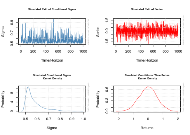
函数 ugarchpath() 模拟由 ugarchspec() 指定的 GARCH 模型。该函数首先需要由 ugarchspec() 创建的指定对象。参数 n.sim 和 n.start 分别指定过程的大小和预热期的长度(分别默认为 1000 和 0。我强烈建议将预热期设置为至少 500,但我设置为 1000)。该函数创建的对象不仅包含模拟序列,还包含残差和 \(\sigma_t\)。
rseed 参数控制函数用于生成数据的随机种子。请注意,此函数会有效地忽略 set.seed(),因此如果需要一致的结果,则需要设置此参数。
这些对象相应的 plot() 方法并不完全透明。它可以创建一些图,当在命令行中对 uGARCHpath 对象调用 plot() 时,系统会提示用户输入与所需图形对应的数字。这有时挺痛苦,所以不要忘记将所需的编号传递给 which 参数以避免提示,设置 which = 2 将正好给出序列的图。
old_par <- par()
par(mfrow = c(2, 2))

x_obj <- ugarchpath(
    spec1, n.sim = 1000, n.start = 1000, rseed = 111217)
show(x_obj)
##
## *------------------------------------*
## *     GARCH Model Path Simulation    *
## *------------------------------------*
## Model: sGARCH
## Horizon:  1000
## Simulations: 1
##                 Seed Sigma2.Mean Sigma2.Min Sigma2.Max Series.Mean
## sim1          111217       0.332      0.251      0.915    0.000165
## Mean(All)          0       0.332      0.251      0.915    0.000165
## Unconditional     NA       0.333         NA         NA    0.000000
##               Series.Min Series.Max
## sim1               -1.76       1.62
## Mean(All)          -1.76       1.62
## Unconditional         NA         NA
for (i in 1:4)
{
    plot(x_obj, which = i)
}
par(old_par)
## Warning in par(old_par): graphical parameter "cin" cannot be set
## Warning in par(old_par): graphical parameter "cra" cannot be set
## Warning in par(old_par): graphical parameter "csi" cannot be set
## Warning in par(old_par): graphical parameter "cxy" cannot be set
## Warning in par(old_par): graphical parameter "din" cannot be set
## Warning in par(old_par): graphical parameter "page" cannot be set
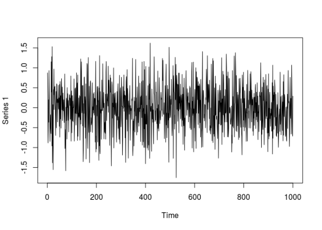
# The actual series
x1 <- x_obj@path$seriesSim
plot.ts(x1)
拟合一个 \(\text{GARCH}(1,1)\) 模型
ugarchfit() 函数拟合 GARCH 模型。该函数需要指定和数据集。solver 参数接受一个字符串,说明要使用哪个数值优化器来寻找参数估计值。函数的大多数参数管理数值优化器的接口。特别是,solver.control 可以接受一个传递给优化器的参数列表。我们稍后会更详细地讨论这个问题。
用于生成模拟数据的指定将不适用于 ugarchfit(),因为它包含其参数的固定值。在我的情况下,我将需要创建第二个指定对象。
spec <- ugarchspec(
    mean.model = list(armaOrder = c(0, 0), include.mean = FALSE))
fit <- ugarchfit(spec, data = x1)
show(fit)
##
## *---------------------------------*
## *          GARCH Model Fit        *
## *---------------------------------*
##
## Conditional Variance Dynamics
## -----------------------------------
## GARCH Model  : sGARCH(1,1)
## Mean Model   : ARFIMA(0,0,0)
## Distribution : norm
##
## Optimal Parameters
## ------------------------------------
##         Estimate  Std. Error    t value Pr(>|t|)
## omega   0.000713    0.001258    0.56696  0.57074
## alpha1  0.002905    0.003714    0.78206  0.43418
## beta1   0.994744    0.000357 2786.08631  0.00000
##
## Robust Standard Errors:
##         Estimate  Std. Error    t value Pr(>|t|)
## omega   0.000713    0.001217    0.58597  0.55789
## alpha1  0.002905    0.003661    0.79330  0.42760
## beta1   0.994744    0.000137 7250.45186  0.00000
##
## LogLikelihood : -860.486
##
## Information Criteria
## ------------------------------------
##
## Akaike       1.7270
## Bayes        1.7417
## Shibata      1.7270
## Hannan-Quinn 1.7326
##
## Weighted Ljung-Box Test on Standardized Residuals
## ------------------------------------
##                         statistic p-value
## Lag[1]                      3.998 0.04555
## Lag[2*(p+q)+(p+q)-1][2]     4.507 0.05511
## Lag[4*(p+q)+(p+q)-1][5]     9.108 0.01555
## d.o.f=0
## H0 : No serial correlation
##
## Weighted Ljung-Box Test on Standardized Squared Residuals
## ------------------------------------
##                         statistic   p-value
## Lag[1]                      29.12 6.786e-08
## Lag[2*(p+q)+(p+q)-1][5]     31.03 1.621e-08
## Lag[4*(p+q)+(p+q)-1][9]     32.26 1.044e-07
## d.o.f=2
##
## Weighted ARCH LM Tests
## ------------------------------------
##             Statistic Shape Scale P-Value
## ARCH Lag[3]     1.422 0.500 2.000  0.2331
## ARCH Lag[5]     2.407 1.440 1.667  0.3882
## ARCH Lag[7]     2.627 2.315 1.543  0.5865
##
## Nyblom stability test
## ------------------------------------
## Joint Statistic:  0.9518
## Individual Statistics:
## omega  0.3296
## alpha1 0.2880
## beta1  0.3195
##
## Asymptotic Critical Values (10% 5% 1%)
## Joint Statistic:          0.846 1.01 1.35
## Individual Statistic:     0.35 0.47 0.75
##
## Sign Bias Test
## ------------------------------------
##                    t-value      prob sig
## Sign Bias           0.3946 6.933e-01
## Negative Sign Bias  3.2332 1.264e-03 ***
## Positive Sign Bias  4.2142 2.734e-05 ***
## Joint Effect       28.2986 3.144e-06 ***
##
##
## Adjusted Pearson Goodness-of-Fit Test:
## ------------------------------------
##   group statistic p-value(g-1)
## 1    20     20.28       0.3779
## 2    30     26.54       0.5965
## 3    40     36.56       0.5817
## 4    50     47.10       0.5505
##
##
## Elapsed time : 2.60606
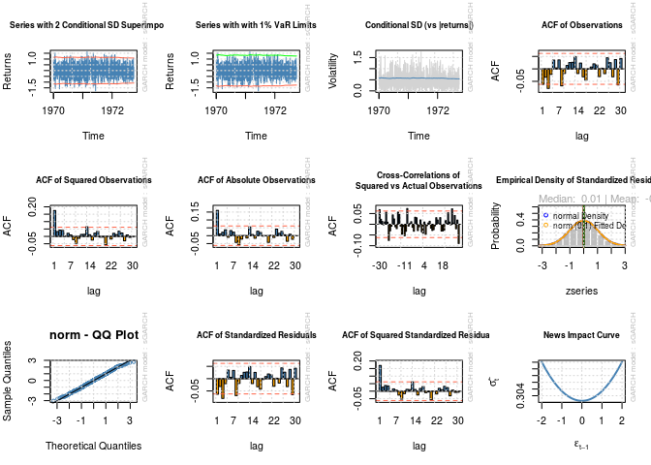
par(mfrow = c(3, 4))
for (i in 1:12)
{
    plot(fit, which = i)
}
##
## please wait...calculating quantiles...
par(old_par)
## Warning in par(old_par): graphical parameter "cin" cannot be set
## Warning in par(old_par): graphical parameter "cra" cannot be set
## Warning in par(old_par): graphical parameter "csi" cannot be set
## Warning in par(old_par): graphical parameter "cxy" cannot be set
## Warning in par(old_par): graphical parameter "din" cannot be set
## Warning in par(old_par): graphical parameter "page" cannot be set
注意估计的参数和标准差?即使对于 1000 的样本大小,估计也与“正确”数字相去甚远,并且基于估计标准差的合理置信区间不包含正确的值。看起来我在上一篇文章中记录的问题并没有消失。
出于好奇,在 Prof. Santos 建议范围的其他指定会发生什么?
x_obj <- ugarchpath(
    spec2, n.start = 1000, rseed = 111317)
x2 <- x_obj@path$seriesSim
fit <- ugarchfit(spec, x2)
show(fit)
##
## *---------------------------------*
## *          GARCH Model Fit        *
## *---------------------------------*
##
## Conditional Variance Dynamics
## -----------------------------------
## GARCH Model  : sGARCH(1,1)
## Mean Model   : ARFIMA(0,0,0)
## Distribution : norm
##
## Optimal Parameters
## ------------------------------------
##         Estimate  Std. Error    t value Pr(>|t|)
## omega   0.001076    0.002501    0.43025  0.66701
## alpha1  0.001992    0.002948    0.67573  0.49921
## beta1   0.997008    0.000472 2112.23364  0.00000
##
## Robust Standard Errors:
##         Estimate  Std. Error    t value Pr(>|t|)
## omega   0.001076    0.002957    0.36389  0.71594
## alpha1  0.001992    0.003510    0.56767  0.57026
## beta1   0.997008    0.000359 2777.24390  0.00000
##
## LogLikelihood : -1375.951
##
## Information Criteria
## ------------------------------------
##
## Akaike       2.7579
## Bayes        2.7726
## Shibata      2.7579
## Hannan-Quinn 2.7635
##
## Weighted Ljung-Box Test on Standardized Residuals
## ------------------------------------
##                         statistic p-value
## Lag[1]                     0.9901  0.3197
## Lag[2*(p+q)+(p+q)-1][2]    1.0274  0.4894
## Lag[4*(p+q)+(p+q)-1][5]    3.4159  0.3363
## d.o.f=0
## H0 : No serial correlation
##
## Weighted Ljung-Box Test on Standardized Squared Residuals
## ------------------------------------
##                         statistic p-value
## Lag[1]                      3.768 0.05226
## Lag[2*(p+q)+(p+q)-1][5]     4.986 0.15424
## Lag[4*(p+q)+(p+q)-1][9]     7.473 0.16272
## d.o.f=2
##
## Weighted ARCH LM Tests
## ------------------------------------
##             Statistic Shape Scale P-Value
## ARCH Lag[3]    0.2232 0.500 2.000  0.6366
## ARCH Lag[5]    0.4793 1.440 1.667  0.8897
## ARCH Lag[7]    2.2303 2.315 1.543  0.6686
##
## Nyblom stability test
## ------------------------------------
## Joint Statistic:  0.3868
## Individual Statistics:
## omega  0.2682
## alpha1 0.2683
## beta1  0.2669
##
## Asymptotic Critical Values (10% 5% 1%)
## Joint Statistic:          0.846 1.01 1.35
## Individual Statistic:     0.35 0.47 0.75
##
## Sign Bias Test
## ------------------------------------
##                    t-value   prob sig
## Sign Bias           0.5793 0.5625
## Negative Sign Bias  1.3358 0.1819
## Positive Sign Bias  1.5552 0.1202
## Joint Effect        5.3837 0.1458
##
##
## Adjusted Pearson Goodness-of-Fit Test:
## ------------------------------------
##   group statistic p-value(g-1)
## 1    20     24.24       0.1871
## 2    30     30.50       0.3894
## 3    40     38.88       0.4753
## 4    50     48.40       0.4974
##
##
## Elapsed time : 2.841597
没有更好。现在让我们看看当我们使用不同的优化算法时会发生什么。
rugarch 中的优化与参数估计
优化器的选择
ugarchfit() 的默认参数很好地找到了我称之为模型 2 的适当参数(其中 \(\alpha = 0.1\) 和 \(\beta = 0.7\)),但不适用于模型 1(\(\alpha = \beta = 0.2\))。我想知道的是何时一个求解器能击败另一个求解器。
正如 Vivek Rao[2] 在 R-SIG-Finance 邮件列表中所说,“最佳”估计是最大化似然函数(或等效地,对数似然函数)的估计,在上一篇文章中我忽略了检查对数似然函数值。在这里,我将看到哪些优化程序导致最大对数似然。
下面是一个辅助函数,它简化了拟合 GARCH 模型参数、提取对数似然、参数值和标准差的过程,同时允许将不同的值传递给 solver 和 solver.control。
evalSolverFit <- function(spec, data,
                          solver = "solnp",
                          solver.control = list())
{
    # Calls ugarchfit(spec, data, solver, solver.control), and returns a vector
    # containing the log likelihood, parameters, and parameter standard errors.
    # Parameters are equivalent to those seen in ugarchfit(). If the solver fails
    # to converge, NA will be returned

    vec <- NA
    tryCatch(
        {
            fit <- ugarchfit(
                spec = spec,
                data = data,
                solver = solver,
                solver.control = solver.control)

            coef_se_names <- paste(
                "se", names(fit@fit$coef), sep = ".")
            se <- fit@fit$se.coef
            names(se) <- coef_se_names

            robust_coef_se_names <- paste(
                "robust.se", names(fit@fit$coef), sep = ".")
            robust.se <- fit@fit$robust.se.coef
            names(robust.se) <- robust_coef_se_names

            vec <- c(fit@fit$coef, se, robust.se)
            vec["LLH"] <- fit@fit$LLH
        },
        error = function(w) { NA })

    return(vec)
}
下面我列出将要考虑的所有优化方案。我只使用 solver.control,但可能有其他参数可以帮助数值优化算法,即 numderiv.control,它们作为控制参数传递给负责标准差计算的数值算法。这利用了包含 numDeriv 的包,它执行数值微分。
solvers <- list(
    # A list of lists where each sublist contains parameters to
    # pass to a solver
    list("solver" = "nlminb", "solver.control" = list()),
    list("solver" = "solnp", "solver.control" = list()),
    list("solver" = "lbfgs", "solver.control" = list()),
    list("solver" = "gosolnp",
         "solver.control" = list("n.restarts" = 100, "n.sim" = 100)),
    list("solver" = "hybrid", "solver.control" = list()),
    list("solver" = "nloptr", "solver.control" = list("solver" = 1)),  # COBYLA
    list("solver" = "nloptr", "solver.control" = list("solver" = 2)),  # BOBYQA
    list("solver" = "nloptr", "solver.control" = list("solver" = 3)),  # PRAXIS
    list("solver" = "nloptr",
         "solver.control" = list("solver" = 4)),  # NELDERMEAD
    list("solver" = "nloptr", "solver.control" = list("solver" = 5)),  # SBPLX
    list("solver" = "nloptr",
         "solver.control" = list("solver" = 6)),  # AUGLAG+COBYLA
    list("solver" = "nloptr",
         "solver.control" = list("solver" = 7)),  # AUGLAG+BOBYQA
    list("solver" = "nloptr",
         "solver.control" = list("solver" = 8)),  # AUGLAG+PRAXIS
    list("solver" = "nloptr",
         "solver.control" = list("solver" = 9)),  # AUGLAG+NELDERMEAD
    list("solver" = "nloptr",
         "solver.control" = list("solver" = 10))  # AUGLAG+SBPLX
)

tags <- c(
    # Names for the above list
    "nlminb",
    "solnp",
    "lbfgs",
    "gosolnp",
    "hybrid",
    "nloptr+COBYLA",
    "nloptr+BOBYQA",
    "nloptr+PRAXIS",
    "nloptr+NELDERMEAD",
    "nloptr+SBPLX",
    "nloptr+AUGLAG+COBYLA",
    "nloptr+AUGLAG+BOBYQA",
    "nloptr+AUGLAG+PRAXIS",
    "nloptr+AUGLAG+NELDERMEAD",
    "nloptr+AUGLAG+SBPLX"
)

names(solvers) <- tags
现在让我们进行优化计算选择的交叉射击(gauntlet),看看哪个算法产生的估计在模型 1 生成的数据上达到最大的对数似然。遗憾的是,lbfgs 方法(Broyden-Fletcher-Goldfarb-Shanno 方法的低存储版本)在这个序列上没有收敛,所以我省略了它。
optMethodCompare <- function(data,
                             spec,
                             solvers)
{
    # Runs all solvers in a list for a dataset
    #
    # Args:
    #   data: An object to pass to ugarchfit's data parameter containing the data
    #         to fit
    #   spec: A specification created by ugarchspec to pass to ugarchfit
    #   solvers: A list of lists containing strings of solvers and a list for
    #            solver.control
    #
    # Return:
    #   A matrix containing the result of the solvers (including parameters, se's,
    #   and LLH)

    model_solutions <- lapply(
        solvers,
        function(s)
        {
            args <- s
            args[["spec"]] <- spec
            args[["data"]] <- data
            res <- do.call(evalSolverFit, args = args)
            return(res)
        })
    model_solutions <- do.call(
        rbind, model_solutions)

    return(model_solutions)
}

round(
    optMethodCompare(
        x1, spec, solvers[c(1:2, 4:15)]), digits = 4)
##                              omega   alpha1    beta1   se.omega   se.alpha1   se.beta1   robust.se.omega   robust.se.alpha1   robust.se.beta1         LLH
## -------------------------  -------  -------  -------  ---------  ----------  ---------  ----------------  -----------------  ----------------  ----------
## nlminb                      0.2689   0.1774   0.0000     0.0787      0.0472     0.2447            0.0890             0.0352            0.2830   -849.6927
## solnp                       0.0007   0.0029   0.9947     0.0013      0.0037     0.0004            0.0012             0.0037            0.0001   -860.4860
## gosolnp                     0.2689   0.1774   0.0000     0.0787      0.0472     0.2446            0.0890             0.0352            0.2828   -849.6927
## hybrid                      0.0007   0.0029   0.9947     0.0013      0.0037     0.0004            0.0012             0.0037            0.0001   -860.4860
## nloptr+COBYLA               0.0006   0.0899   0.9101     0.0039      0.0306     0.0370            0.0052             0.0527            0.0677   -871.5006
## nloptr+BOBYQA               0.0003   0.0907   0.9093     0.0040      0.0298     0.0375            0.0057             0.0532            0.0718   -872.3436
## nloptr+PRAXIS               0.2689   0.1774   0.0000     0.0786      0.0472     0.2444            0.0888             0.0352            0.2823   -849.6927
## nloptr+NELDERMEAD           0.0010   0.0033   0.9935     0.0013      0.0039     0.0004            0.0013             0.0038            0.0001   -860.4845
## nloptr+SBPLX                0.0010   0.1000   0.9000     0.0042      0.0324     0.0386            0.0055             0.0536            0.0680   -872.2736
## nloptr+AUGLAG+COBYLA        0.0006   0.0899   0.9101     0.0039      0.0306     0.0370            0.0052             0.0527            0.0677   -871.5006
## nloptr+AUGLAG+BOBYQA        0.0003   0.0907   0.9093     0.0040      0.0298     0.0375            0.0057             0.0532            0.0718   -872.3412
## nloptr+AUGLAG+PRAXIS        0.1246   0.1232   0.4948     0.0620      0.0475     0.2225            0.0701             0.0439            0.2508   -851.0547
## nloptr+AUGLAG+NELDERMEAD    0.2689   0.1774   0.0000     0.0786      0.0472     0.2445            0.0889             0.0352            0.2826   -849.6927
## nloptr+AUGLAG+SBPLX         0.0010   0.1000   0.9000     0.0042      0.0324     0.0386            0.0055             0.0536            0.0680   -872.2736
根据最大似然准则,“最优”结果是由 gosolnp 实现的。结果有一个不幸的属性——\(\beta \approx 0\),这当然不是正确的,但至少 \(\beta\) 的标准差会创建一个包含 \(\beta\) 真值的置信区间。其中,我的首选估计是由 AUGLAG + PRAXIS 生成的,因为 \(\beta\) 似乎是合理的,事实上估计都接近事实(至少在置信区间包含真值的意义上),但不幸的是,即使它们是最合理的,估计并没有最大化对数似然。
如果我们看一下模型 2,我们会看到什么?同样,lbfgs 没有收敛,所以我省略忽略了它。不幸的是,nlminb 也没有收敛,因此也必须省略。
round(
    optMethodCompare(
        x2, spec, solvers[c(2, 4:15)]), digits = 4)
##                              omega   alpha1    beta1   se.omega   se.alpha1   se.beta1   robust.se.omega   robust.se.alpha1   robust.se.beta1         LLH
## -------------------------  -------  -------  -------  ---------  ----------  ---------  ----------------  -----------------  ----------------  ----------
## solnp                       0.0011   0.0020   0.9970     0.0025      0.0029     0.0005            0.0030             0.0035            0.0004   -1375.951
## gosolnp                     0.0011   0.0020   0.9970     0.0025      0.0029     0.0005            0.0030             0.0035            0.0004   -1375.951
## hybrid                      0.0011   0.0020   0.9970     0.0025      0.0029     0.0005            0.0030             0.0035            0.0004   -1375.951
## nloptr+COBYLA               0.0016   0.0888   0.9112     0.0175      0.0619     0.0790            0.0540             0.2167            0.2834   -1394.529
## nloptr+BOBYQA               0.0010   0.0892   0.9108     0.0194      0.0659     0.0874            0.0710             0.2631            0.3572   -1395.310
## nloptr+PRAXIS               0.5018   0.0739   0.3803     0.3178      0.0401     0.3637            0.2777             0.0341            0.3225   -1373.632
## nloptr+NELDERMEAD           0.0028   0.0026   0.9944     0.0028      0.0031     0.0004            0.0031             0.0035            0.0001   -1375.976
## nloptr+SBPLX                0.0029   0.1000   0.9000     0.0146      0.0475     0.0577            0.0275             0.1108            0.1408   -1395.807
## nloptr+AUGLAG+COBYLA        0.0016   0.0888   0.9112     0.0175      0.0619     0.0790            0.0540             0.2167            0.2834   -1394.529
## nloptr+AUGLAG+BOBYQA        0.0010   0.0892   0.9108     0.0194      0.0659     0.0874            0.0710             0.2631            0.3572   -1395.310
## nloptr+AUGLAG+PRAXIS        0.5018   0.0739   0.3803     0.3178      0.0401     0.3637            0.2777             0.0341            0.3225   -1373.632
## nloptr+AUGLAG+NELDERMEAD    0.0001   0.0000   1.0000     0.0003      0.0003     0.0000            0.0004             0.0004            0.0000   -1375.885
## nloptr+AUGLAG+SBPLX         0.0029   0.1000   0.9000     0.0146      0.0475     0.0577            0.0275             0.1108            0.1408   -1395.807
这里是 PRAXIS 和 AUGLAG + PRAXIS 给出了“最优”结果,只有这两种方法做到了。其他优化器给出了明显糟糕的结果。也就是说,“最优”解在参数为非零、置信区间包含正确值上是首选的。
如果我们将样本限制为 100,会发生什么?(lbfgs 仍然不起作用。)
round(
    optMethodCompare(
        x1[1:100], spec, solvers[c(1:2, 4:15)]), digits = 4)
##                              omega   alpha1    beta1   se.omega   se.alpha1   se.beta1   robust.se.omega   robust.se.alpha1   robust.se.beta1        LLH
## -------------------------  -------  -------  -------  ---------  ----------  ---------  ----------------  -----------------  ----------------  ---------
## nlminb                      0.0451   0.2742   0.5921     0.0280      0.1229     0.1296            0.0191             0.0905            0.0667   -80.6587
## solnp                       0.0451   0.2742   0.5921     0.0280      0.1229     0.1296            0.0191             0.0905            0.0667   -80.6587
## gosolnp                     0.0451   0.2742   0.5921     0.0280      0.1229     0.1296            0.0191             0.0905            0.0667   -80.6587
## hybrid                      0.0451   0.2742   0.5921     0.0280      0.1229     0.1296            0.0191             0.0905            0.0667   -80.6587
## nloptr+COBYLA               0.0007   0.1202   0.8798     0.0085      0.0999     0.0983            0.0081             0.1875            0.1778   -85.3121
## nloptr+BOBYQA               0.0005   0.1190   0.8810     0.0085      0.0994     0.0992            0.0084             0.1892            0.1831   -85.3717
## nloptr+PRAXIS               0.0451   0.2742   0.5921     0.0280      0.1229     0.1296            0.0191             0.0905            0.0667   -80.6587
## nloptr+NELDERMEAD           0.0451   0.2742   0.5920     0.0281      0.1230     0.1297            0.0191             0.0906            0.0667   -80.6587
## nloptr+SBPLX                0.0433   0.2740   0.5998     0.0269      0.1237     0.1268            0.0182             0.0916            0.0648   -80.6616
## nloptr+AUGLAG+COBYLA        0.0007   0.1202   0.8798     0.0085      0.0999     0.0983            0.0081             0.1875            0.1778   -85.3121
## nloptr+AUGLAG+BOBYQA        0.0005   0.1190   0.8810     0.0085      0.0994     0.0992            0.0084             0.1892            0.1831   -85.3717
## nloptr+AUGLAG+PRAXIS        0.0451   0.2742   0.5921     0.0280      0.1229     0.1296            0.0191             0.0905            0.0667   -80.6587
## nloptr+AUGLAG+NELDERMEAD    0.0451   0.2742   0.5921     0.0280      0.1229     0.1296            0.0191             0.0905            0.0667   -80.6587
## nloptr+AUGLAG+SBPLX         0.0450   0.2742   0.5924     0.0280      0.1230     0.1295            0.0191             0.0906            0.0666   -80.6587
round(
    optMethodCompare(
        x2[1:100], spec, solvers[c(1:2, 4:15)]), digits = 4)
##                              omega   alpha1    beta1   se.omega   se.alpha1   se.beta1   robust.se.omega   robust.se.alpha1   robust.se.beta1         LLH
## -------------------------  -------  -------  -------  ---------  ----------  ---------  ----------------  -----------------  ----------------  ----------
## nlminb                      0.7592   0.0850   0.0000     2.1366      0.4813     3.0945            7.5439             1.7763           11.0570   -132.4614
## solnp                       0.0008   0.0000   0.9990     0.0291      0.0417     0.0066            0.0232             0.0328            0.0034   -132.9182
## gosolnp                     0.0537   0.0000   0.9369     0.0521      0.0087     0.0713            0.0430             0.0012            0.0529   -132.9124
## hybrid                      0.0008   0.0000   0.9990     0.0291      0.0417     0.0066            0.0232             0.0328            0.0034   -132.9182
## nloptr+COBYLA               0.0014   0.0899   0.9101     0.0259      0.0330     0.1192            0.0709             0.0943            0.1344   -135.7495
## nloptr+BOBYQA               0.0008   0.0905   0.9095     0.0220      0.0051     0.1145            0.0687             0.0907            0.1261   -135.8228
## nloptr+PRAXIS               0.0602   0.0000   0.9293     0.0522      0.0088     0.0773            0.0462             0.0015            0.0565   -132.9125
## nloptr+NELDERMEAD           0.0024   0.0000   0.9971     0.0473      0.0629     0.0116            0.0499             0.0680            0.0066   -132.9186
## nloptr+SBPLX                0.0027   0.1000   0.9000     0.0238      0.0493     0.1308            0.0769             0.1049            0.1535   -135.9175
## nloptr+AUGLAG+COBYLA        0.0014   0.0899   0.9101     0.0259      0.0330     0.1192            0.0709             0.0943            0.1344   -135.7495
## nloptr+AUGLAG+BOBYQA        0.0008   0.0905   0.9095     0.0221      0.0053     0.1145            0.0687             0.0907            0.1262   -135.8226
## nloptr+AUGLAG+PRAXIS        0.0602   0.0000   0.9294     0.0523      0.0090     0.0771            0.0462             0.0014            0.0565   -132.9125
## nloptr+AUGLAG+NELDERMEAD    0.0000   0.0000   0.9999     0.0027      0.0006     0.0005            0.0013             0.0004            0.0003   -132.9180
## nloptr+AUGLAG+SBPLX         0.0027   0.1000   0.9000     0.0238      0.0493     0.1308            0.0769             0.1049            0.1535   -135.9175
结果并不令人兴奋。多个求解器获得了模型 1 生成序列的“最佳”结果,同时 \(\omega\) 的 95% 置信区间(CI)不包含 \(\omega\) 的真实值,尽管其他的 CI 将包含其真实值。对于由模型 2 生成的序列,最佳结果是由 nlminb 求解器实现的,但参数值不合理,标准差很大。至少 CI 将包含正确值。
从这里开始,我们不应再仅仅关注两个序列,而是在两个模型生成的许多模拟序列中研究这些方法的表现。这篇文章中的模拟对于我的笔记本电脑而言计算量太大,因此我将使用我院系的超级计算机来执行它们,利用其多核进行并行计算。
library(foreach)
library(doParallel)

logfile <- ""

# logfile <- "outfile.log"
# if (!file.exists(logfile)) {
#   file.create(logfile)
# }

cl <- makeCluster(
    detectCores() - 1, outfile = logfile)
registerDoParallel(cl)

optMethodSims <- function(
    gen_spec,
    n.sim = 1000,
    m.sim = 1000,
    fit_spec = ugarchspec(
        mean.model = list(
            armaOrder = c(0,0), include.mean = FALSE)),
    solvers = list(
        "solnp" = list(
            "solver" = "solnp", "solver.control" = list())),
    rseed = NA, verbose = FALSE)
{
    # Performs simulations in parallel of GARCH processes via rugarch and returns
    # a list with the results of different optimization routines
    #
    # Args:
    #   gen_spec: The specification for generating a GARCH sequence, produced by
    #             ugarchspec
    #   n.sim: An integer denoting the length of the simulated series
    #   m.sim: An integer for the number of simulated sequences to generate
    #   fit_spec: A ugarchspec specification for the model to fit
    #   solvers: A list of lists containing strings of solvers and a list for
    #            solver.control
    #   rseed: Optional seeding value(s) for the random number generator. For
    #          m.sim>1, it is possible to provide either a single seed to
    #          initialize all values, or one seed per separate simulation (i.e.
    #          m.sim seeds). However, in the latter case this may result in some
    #          slight overhead depending on how large m.sim is
    #   verbose: Boolean for whether to write data tracking the progress of the
    #            loop into an output file
    #   outfile: A string for the file to store verbose output to (relevant only
    #            if verbose is TRUE)
    #
    # Return:
    #   A list containing the result of calling optMethodCompare on each generated
    #   sequence

    fits <- foreach(
        i = 1:m.sim,
        .packages = c("rugarch"),
        .export = c(
            "optMethodCompare", "evalSolverFit")) %dopar%
            {
                if (is.na(rseed))
                {
                    newseed <- NA
                }
                else if (is.vector(rseed))
                {
                    newseed <- rseed[i]
                }
                else
                {
                    newseed <- rseed + i - 1
                }

                if (verbose)
                {
                    cat(as.character(Sys.time()), ": Now on simulation ", i, "\n")
                }

                sim <- ugarchpath(
                    gen_spec, n.sim = n.sim, n.start = 1000,
                    m.sim = 1, rseed = newseed)
                x <- sim@path$seriesSim
                optMethodCompare(
                    x, spec = fit_spec, solvers = solvers)
            }

    return(fits)
}

# Specification 1 first
spec1_n100 <- optMethodSims(
    spec1, n.sim = 100, m.sim = 1000,
    solvers = solvers, verbose = TRUE)
spec1_n500 <- optMethodSims(
    spec1, n.sim = 500, m.sim = 1000,
    solvers = solvers, verbose = TRUE)
spec1_n1000 <- optMethodSims(
    spec1, n.sim = 1000, m.sim = 1000,
    solvers = solvers, verbose = TRUE)

# Specification 2 next
spec2_n100 <- optMethodSims(
    spec2, n.sim = 100, m.sim = 1000,
    solvers = solvers, verbose = TRUE)
spec2_n500 <- optMethodSims(
    spec2, n.sim = 500, m.sim = 1000,
    solvers = solvers, verbose = TRUE)
spec2_n1000 <- optMethodSims(
    spec2, n.sim = 1000, m.sim = 1000,
    solvers = solvers, verbose = TRUE)
以下是一组辅助函数,用于我要进行的分析。
optMethodSims_getAllVals <- function(param,
                                     solver,
                                     reslist)
{
    # Get all values for a parameter obtained by a certain solver after getting a
    # list of results via optMethodSims
    #
    # Args:
    #   param: A string for the parameter to get (such as "beta1")
    #   solver: A string for the solver for which to get the parameter (such as
    #           "nlminb")
    #   reslist: A list created by optMethodSims
    #
    # Return:
    #   A vector of values of the parameter for each simulation

    res <- sapply(
        reslist,
        function(l)
        {
            return(l[solver, param])
        })

    return(res)
}

optMethodSims_getBestVals <- function(reslist,
                                      opt_vec = TRUE,
                                      reslike = FALSE)
{
    # A function that gets the optimizer that maximized the likelihood function
    # for each entry in reslist
    #
    # Args:
    #   reslist: A list created by optMethodSims
    #   opt_vec: A boolean indicating whether to return a vector with the name of
    #            the optimizers that maximized the log likelihood
    #   reslike: A bookean indicating whether the resulting list should consist of
    #            matrices of only one row labeled "best" with a structure like
    #            reslist
    #
    # Return:
    #   If opt_vec is TRUE, a list of lists, where each sublist contains a vector
    #   of strings naming the opimizers that maximized the likelihood function and
    #   a matrix of the parameters found. Otherwise, just the matrix (resembles
    #   the list generated by optMethodSims)

    res <- lapply(
        reslist,
        function(l)
        {
            max_llh <- max(l[, "LLH"], na.rm = TRUE)
            best_idx <- (l[, "LLH"] == max_llh) & (!is.na(l[, "LLH"]))
            best_mat <- l[best_idx, , drop = FALSE]

            if (opt_vec)
            {
                return(
                    list(
                        "solvers" = rownames(best_mat), "params" = best_mat))
            }
            else
            {
                return(best_mat)
            }
        })

    if (reslike)
    {
        res <- lapply(
            res,
            function(l)
            {
                mat <- l$params[1, , drop = FALSE]
                rownames(mat) <- "best"
                return(mat)
            })
    }

    return(res)
}

optMethodSims_getCaptureRate <- function(param,
                                         solver,
                                         reslist,
                                         multiplier = 2,
                                         spec,
                                         use_robust = TRUE)
{
    # Gets the rate a confidence interval for a parameter captures the true value
    #
    # Args:
    #   param: A string for the parameter being worked with
    #   solver: A string for the solver used to estimate the parameter
    #   reslist: A list created by optMethodSims
    #   multiplier: A floating-point number for the multiplier to the standard
    #               error, appropriate for the desired confidence level
    #   spec: A ugarchspec specification with the fixed parameters containing the
    #         true parameter value
    #   use_robust: Use robust standard errors for computing CIs
    #
    # Return:
    #   A float for the proportion of times the confidence interval captured the
    #   true parameter value

    se_string <- ifelse(
        use_robust, "robust.se.", "se.")

    est <- optMethodSims_getAllVals(
        param, solver, reslist)
    moe_est <- multiplier * optMethodSims_getAllVals(
        paste0(se_string, param), solver, reslist)
    param_val <- spec@model$fixed.pars[[param]]
    contained <- (param_val <= est + moe_est) & (param_val >= est - moe_est)
    return(mean(contained, na.rm = TRUE))
}

optMethodSims_getMaxRate <- function(solver,
                                     maxlist)
{
    # Gets how frequently a solver found a maximal log likelihood
    #
    # Args:
    #   solver: A string for the solver
    #   maxlist A list created by optMethodSims_getBestVals with entries
    #           containing vectors naming the solvers that maximized the log
    #           likelihood
    #
    # Return:
    #   The proportion of times the solver maximized the log likelihood

    maxed <- sapply(
        maxlist,
        function(l)
        {
            solver %in% l$solvers
        })

    return(mean(maxed))
}

optMethodSims_getFailureRate <- function(solver,
                                         reslist)
{
    # Computes the proportion of times a solver failed to converge.
    #
    # Args:
    #   solver: A string for the solver
    #   reslist: A list created by optMethodSims
    #
    # Return:
    #   Numeric proportion of times a solver failed to converge

    failed <- sapply(
        reslist,
        function(l)
        {
            is.na(l[solver, "LLH"])
        })

    return(mean(failed))
}

# Vectorization
optMethodSims_getCaptureRate <- Vectorize(
    optMethodSims_getCaptureRate, vectorize.args = "solver")
optMethodSims_getMaxRate <- Vectorize(
    optMethodSims_getMaxRate, vectorize.args = "solver")
optMethodSims_getFailureRate <- Vectorize(
    optMethodSims_getFailureRate, vectorize.args = "solver")
我首先为固定样本量和模型创建表:
- 所有求解器中,某个求解器达到最高对数似然的频率
- 某个求解器未能收敛的频率
- 基于某个求解器的解,95% 置信区间包含每个参数真实值的频率(称为“捕获率”,并使用稳健标准差)
solver_table <- function(reslist,
                         tags,
                         spec)
{
    # Creates a table describing important solver statistics
    #
    # Args:
    #   reslist: A list created by optMethodSims
    #   tags: A vector with strings naming all solvers to include in the table
    #   spec: A ugarchspec specification with the fixed parameters containing the
    #         true parameter value
    #
    # Return:
    #   A matrix containing metrics describing the performance of the solvers

    params <- names(spec1@model$fixed.pars)

    max_rate <- optMethodSims_getMaxRate(
        tags, optMethodSims_getBestVals(reslist))
    failure_rate <- optMethodSims_getFailureRate(
        tags, reslist)
    capture_rate <- lapply(
        params,
        function(p)
        {
            optMethodSims_getCaptureRate(
                p, tags, reslist, spec = spec)
        })

    return_mat <- cbind(
        "Maximization Rate" = max_rate,
        "Failure Rate" = failure_rate)

    capture_mat <- do.call(cbind, capture_rate)
    colnames(capture_mat) <- paste(
        params, "95% CI Capture Rate")

    return_mat <- cbind(
        return_mat, capture_mat)

    return(return_mat)
}
- Model 1, \(n=100\)
as.data.frame(
    round(
        solver_table(spec1_n100, tags, spec1) * 100,
        digits = 1))
##                             Maximization Rate   Failure Rate   omega 95% CI Capture Rate   alpha1 95% CI Capture Rate   beta1 95% CI Capture Rate
## -------------------------  ------------------  -------------  --------------------------  ---------------------------  --------------------------
## nlminb                                   16.2           20.0                        21.8                         29.2                        24.0
## solnp                                     0.1            0.0                        13.7                         24.0                        15.4
## lbfgs                                    15.1           35.2                        56.6                         67.9                        58.0
## gosolnp                                  20.3            0.0                        20.3                         32.6                        21.9
## hybrid                                    0.1            0.0                        13.7                         24.0                        15.4
## nloptr+COBYLA                             0.0            0.0                         6.3                         82.6                        19.8
## nloptr+BOBYQA                             0.0            0.0                         5.4                         82.1                        18.5
## nloptr+PRAXIS                            15.8            0.0                        42.1                         54.5                        44.1
## nloptr+NELDERMEAD                         0.4            0.0                         5.7                         19.3                         8.1
## nloptr+SBPLX                              0.1            0.0                         7.7                         85.7                        24.1
## nloptr+AUGLAG+COBYLA                      0.0            0.0                         6.1                         84.5                        19.9
## nloptr+AUGLAG+BOBYQA                      0.1            0.0                         6.5                         83.2                        19.4
## nloptr+AUGLAG+PRAXIS                     22.6            0.0                        41.2                         54.6                        44.1
## nloptr+AUGLAG+NELDERMEAD                 11.1            0.0                         7.5                         18.8                         9.7
## nloptr+AUGLAG+SBPLX                       0.6            0.0                         7.9                         86.5                        23.0
- Model 1, \(n=500\)
as.data.frame(
    round(
        solver_table(spec1_n500, tags, spec1) * 100,
        digits = 1))
##                             Maximization Rate   Failure Rate   omega 95% CI Capture Rate   alpha1 95% CI Capture Rate   beta1 95% CI Capture Rate
## -------------------------  ------------------  -------------  --------------------------  ---------------------------  --------------------------
## nlminb                                   21.2            0.4                        63.3                         67.2                        63.8
## solnp                                     0.1            0.2                        32.2                         35.6                        32.7
## lbfgs                                     4.5           41.3                        85.0                         87.6                        85.7
## gosolnp                                  35.1            0.0                        69.0                         73.2                        69.5
## hybrid                                    0.1            0.0                        32.3                         35.7                        32.8
## nloptr+COBYLA                             0.0            0.0                         3.2                         83.3                        17.8
## nloptr+BOBYQA                             0.0            0.0                         3.5                         81.5                        18.1
## nloptr+PRAXIS                            18.0            0.0                        83.9                         87.0                        84.2
## nloptr+NELDERMEAD                         0.0            0.0                        16.4                         20.7                        16.7
## nloptr+SBPLX                              0.1            0.0                         3.7                         91.4                        15.7
## nloptr+AUGLAG+COBYLA                      0.0            0.0                         3.2                         83.3                        17.8
## nloptr+AUGLAG+BOBYQA                      0.0            0.0                         3.5                         81.5                        18.1
## nloptr+AUGLAG+PRAXIS                     21.9            0.0                        80.2                         87.4                        83.4
## nloptr+AUGLAG+NELDERMEAD                  0.6            0.0                        20.0                         24.0                        20.5
## nloptr+AUGLAG+SBPLX                       0.0            0.0                         3.7                         91.4                        15.7
- Model 1, \(n=1000\)
as.data.frame(
    round(
        solver_table(spec1_n1000, tags, spec1) * 100,
        digits = 1))
##                             Maximization Rate   Failure Rate   omega 95% CI Capture Rate   alpha1 95% CI Capture Rate   beta1 95% CI Capture Rate
## -------------------------  ------------------  -------------  --------------------------  ---------------------------  --------------------------
## nlminb                                   21.5            0.1                        88.2                         86.1                        87.8
## solnp                                     0.4            0.2                        54.9                         53.6                        54.6
## lbfgs                                     1.1           44.8                        91.5                         88.0                        91.8
## gosolnp                                  46.8            0.0                        87.2                         85.1                        87.0
## hybrid                                    0.5            0.0                        55.0                         53.6                        54.7
## nloptr+COBYLA                             0.0            0.0                         4.1                         74.5                        15.0
## nloptr+BOBYQA                             0.0            0.0                         3.6                         74.3                        15.9
## nloptr+PRAXIS                            17.7            0.0                        92.6                         90.2                        92.2
## nloptr+NELDERMEAD                         0.0            0.0                        30.5                         29.6                        30.9
## nloptr+SBPLX                              0.0            0.0                         3.0                         82.3                        11.6
## nloptr+AUGLAG+COBYLA                      0.0            0.0                         4.1                         74.5                        15.0
## nloptr+AUGLAG+BOBYQA                      0.0            0.0                         3.6                         74.3                        15.9
## nloptr+AUGLAG+PRAXIS                     13.0            0.0                        83.4                         93.9                        86.7
## nloptr+AUGLAG+NELDERMEAD                  0.0            0.0                        34.6                         33.8                        35.0
## nloptr+AUGLAG+SBPLX                       0.0            0.0                         3.0                         82.3                        11.6
- Model 2, \(n=100\)
as.data.frame(
    round(
        solver_table(spec2_n100, tags, spec2) * 100,
        digits = 1))
##                             Maximization Rate   Failure Rate   omega 95% CI Capture Rate   alpha1 95% CI Capture Rate   beta1 95% CI Capture Rate
## -------------------------  ------------------  -------------  --------------------------  ---------------------------  --------------------------
## nlminb                                    8.2           24.2                        22.3                         34.7                        23.9
## solnp                                     0.3            0.0                        21.1                         32.6                        21.3
## lbfgs                                    11.6           29.5                        74.9                         73.2                        70.4
## gosolnp                                  19.0            0.0                        31.9                         41.2                        30.8
## hybrid                                    0.3            0.0                        21.1                         32.6                        21.3
## nloptr+COBYLA                             0.0            0.0                        20.5                         94.7                        61.7
## nloptr+BOBYQA                             0.2            0.0                        19.3                         95.8                        62.2
## nloptr+PRAXIS                            16.0            0.0                        70.2                         57.2                        52.8
## nloptr+NELDERMEAD                         0.2            0.0                         7.8                         27.8                        14.1
## nloptr+SBPLX                              0.1            0.0                        24.9                         91.0                        65.0
## nloptr+AUGLAG+COBYLA                      0.0            0.0                        21.2                         95.1                        62.5
## nloptr+AUGLAG+BOBYQA                      0.9            0.0                        20.1                         96.2                        62.5
## nloptr+AUGLAG+PRAXIS                     38.8            0.0                        70.4                         57.2                        52.7
## nloptr+AUGLAG+NELDERMEAD                 14.4            0.0                        10.7                         26.0                        16.1
## nloptr+AUGLAG+SBPLX                       0.1            0.0                        25.8                         91.9                        65.5
- Model 2, \(n=500\)
as.data.frame(
    round(
        solver_table(spec2_n500, tags, spec2) * 100,
        digits = 1))
##                             Maximization Rate   Failure Rate   omega 95% CI Capture Rate   alpha1 95% CI Capture Rate   beta1 95% CI Capture Rate
## -------------------------  ------------------  -------------  --------------------------  ---------------------------  --------------------------
## nlminb                                    1.7            1.6                        35.0                         37.2                        34.2
## solnp                                     0.1            0.2                        46.2                         48.6                        45.3
## lbfgs                                     2.2           38.4                        85.2                         88.1                        82.3
## gosolnp                                   5.2            0.0                        74.9                         77.8                        72.7
## hybrid                                    0.1            0.0                        46.1                         48.5                        45.2
## nloptr+COBYLA                             0.0            0.0                         8.2                        100.0                        40.5
## nloptr+BOBYQA                             0.0            0.0                         9.5                        100.0                        41.0
## nloptr+PRAXIS                            17.0            0.0                        83.8                         85.1                        81.0
## nloptr+NELDERMEAD                         0.0            0.0                        26.9                         38.2                        27.0
## nloptr+SBPLX                              0.0            0.0                         8.2                        100.0                        40.2
## nloptr+AUGLAG+COBYLA                      0.0            0.0                         8.2                        100.0                        40.5
## nloptr+AUGLAG+BOBYQA                      0.0            0.0                         9.5                        100.0                        41.0
## nloptr+AUGLAG+PRAXIS                     77.8            0.0                        84.4                         85.4                        81.3
## nloptr+AUGLAG+NELDERMEAD                  1.1            0.0                        32.5                         40.3                        32.3
## nloptr+AUGLAG+SBPLX                       0.0            0.0                         8.2                        100.0                        40.2
- Model 2, \(n=1000\)
as.data.frame(
    round(
        solver_table(spec2_n1000, tags, spec2) * 100,
        digits = 1))
##                             Maximization Rate   Failure Rate   omega 95% CI Capture Rate   alpha1 95% CI Capture Rate   beta1 95% CI Capture Rate
## -------------------------  ------------------  -------------  --------------------------  ---------------------------  --------------------------
## nlminb                                    2.7            0.7                        64.1                         68.0                        63.8
## solnp                                     0.0            0.0                        70.1                         73.8                        69.8
## lbfgs                                     0.0           43.4                        90.6                         91.5                        89.9
## gosolnp                                   3.2            0.0                        87.5                         90.3                        86.9
## hybrid                                    0.0            0.0                        70.1                         73.8                        69.8
## nloptr+COBYLA                             0.0            0.0                         2.3                        100.0                        20.6
## nloptr+BOBYQA                             0.0            0.0                         2.5                        100.0                        22.6
## nloptr+PRAXIS                            14.1            0.0                        89.1                         91.3                        88.5
## nloptr+NELDERMEAD                         0.0            0.0                        46.3                         55.6                        45.4
## nloptr+SBPLX                              0.0            0.0                         2.2                        100.0                        19.5
## nloptr+AUGLAG+COBYLA                      0.0            0.0                         2.3                        100.0                        20.6
## nloptr+AUGLAG+BOBYQA                      0.0            0.0                         2.5                        100.0                        22.6
## nloptr+AUGLAG+PRAXIS                     85.5            0.0                        89.1                         91.3                        88.5
## nloptr+AUGLAG+NELDERMEAD                  0.3            0.0                        51.9                         58.2                        51.3
## nloptr+AUGLAG+SBPLX                       0.0            0.0                         2.2                        100.0                        19.5
这些表已经揭示了很多信息。一般来说,NLOpt 中提供的 AUGLAG-PRAXIS 方法(使用主轴求解器的增广拉格朗日方法)似乎对模型 2 最有效,特别是对于大样本;而对于模型 1,gosolnp 方法(使用 Yinyu Ye 的 solnp 求解器,但使用随机初始化和重启)似乎在大样本上胜出。
然而,更大的故事是任何方法都不能成为“最佳”,特别是在样本量较小的情况下。有些优化器始终未能达到最大对数似然,没有优化器能够始终如一地获得最佳结果。此外,不同的优化器似乎在不同的模型下表现更好。真实世界的数据——真正的模型参数从未被知道——暗示了要尝试每个优化器(或至少那些有可能最大化对数似然的),并选择产生最大对数似然的结果。没有算法值得信赖,都无法成为首选算法。
现在让我们看一下参数估计的分布图。首先是辅助函数。
library(ggplot2)

solver_density_plot <- function(param,
                                tags,
                                list_reslist,
                                sample_sizes,
                                spec)
{
    # Given a parameter, creates a density plot for each solver's distribution
    # at different sample sizes
    #
    # Args:
    #   param: A string for the parameter to plot
    #   tags: A character vector containing the solver names
    #   list_reslist: A list of lists created by optMethodSimsf, one for each
    #                 sample size
    #   sample_sizes: A numeric vector identifying the sample size corresponding
    #                 to each object in the above list
    #   spec: A ugarchspec object containing the specification that generated the
    #         datasets
    #
    # Returns:
    #   A ggplot object containing the plot generated

    p <- spec@model$fixed.pars[[param]]
    nlist <- lapply(
        list_reslist,
        function(l)
        {
            optlist <- lapply(
                tags,
                function(t)
                {
                    return(
                        na.omit(
                            optMethodSims_getAllVals(param, t, l)))
                })
            names(optlist) <- tags
            df <- stack(optlist)
            names(df) <- c("param", "optimizer")

            return(df)
        })
    ndf <- do.call(rbind, nlist)
    ndf$n <- rep(
        sample_sizes, times = sapply(nlist, nrow))

    ggplot(
        ndf, aes(x = param)) +
        geom_density(
            fill = "black", alpha = 0.5) +
        geom_vline(
            xintercept = p, color = "blue") +
        facet_grid(
            optimizer ~ n, scales = "free_y")
}
开始画图。
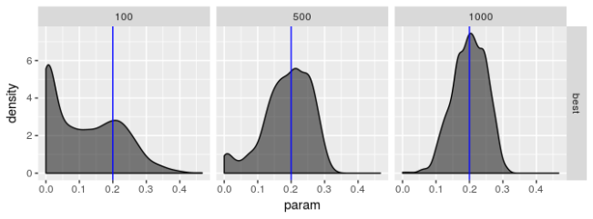
- \(\omega\) 估计,model 1
solver_density_plot(
    "omega", tags,
    list(spec1_n100, spec1_n500, spec1_n1000),
    c(100, 500, 1000), spec1)

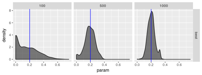
- \(\alpha\) 估计,model 1
solver_density_plot(
    "alpha1", tags,
    list(spec1_n100, spec1_n500, spec1_n1000),
    c(100, 500, 1000), spec1)
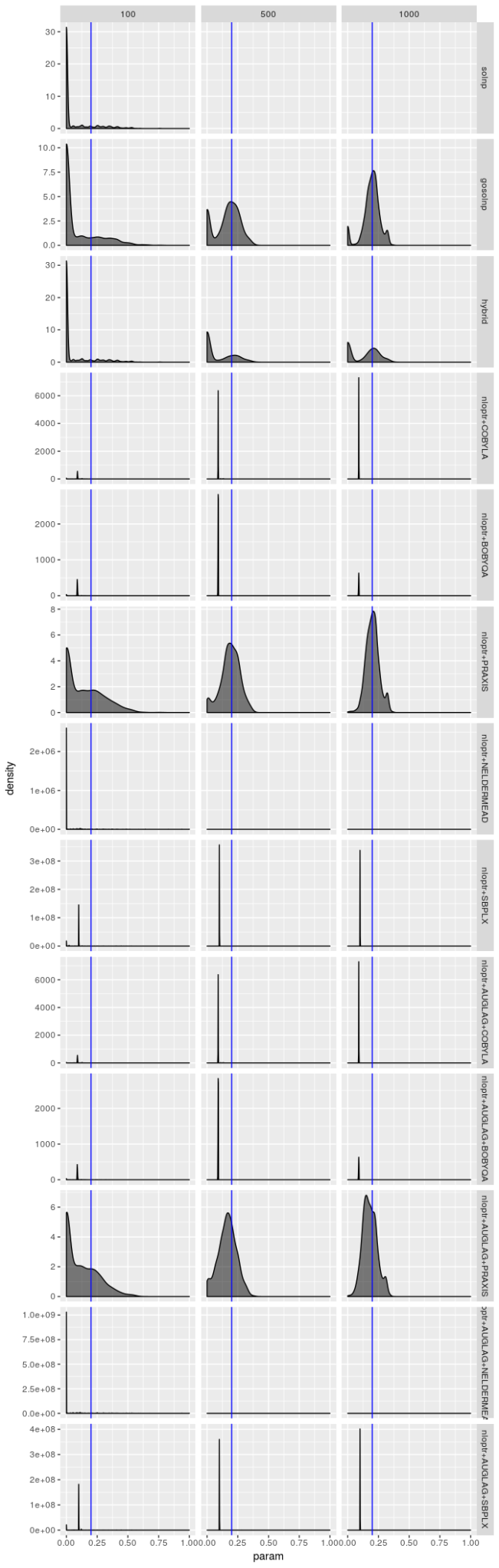
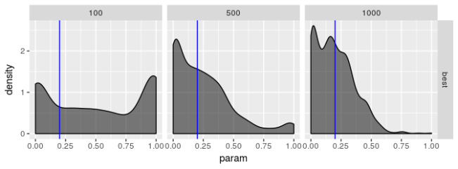
- \(\beta\) 估计,model 1
solver_density_plot(
    "beta1", tags,
    list(spec1_n100, spec1_n500, spec1_n1000),
    c(100, 500, 1000), spec1)
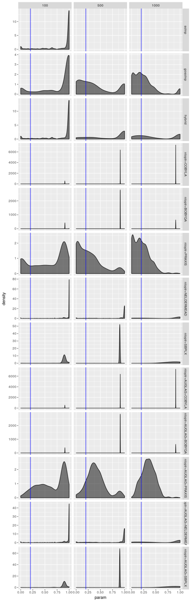
请记住,只有 1000 个模拟序列,并且优化器为每个序列生成解,因此原则上优化器结果不应该是独立的,但优化器运行得非常糟糕的时候,这些密度图才看起来是相同的。但即使优化器的表现不是很糟糕(就像 gosolnp、PRAXIS 和 AUGLAG-PRAXIS 方法的情况一样),有证据表明估计 \(\omega\) 和 \(\alpha\) 的估计错误地接近 0,并且 \(\beta\) 的估计错误地接近 1。对于较小的样本,这些错误更明显。也就是说,对于更好的优化器,估计应该看起来几乎无偏,特别是对于 \(\omega\) 和 \(\alpha\),但是即使对于大样本,它们的变动范围也很大,特别是对于 \(\beta\) 的估计。但是,对于 AUGLAG-PRAXIS 优化器来说情况并非如此,它似乎产生有偏的估计。
让我们看看模型 2 的图。
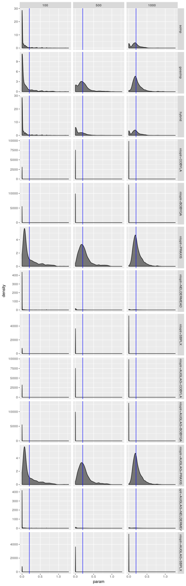
- \(\omega\) 估计,model 2
solver_density_plot(
    "omega", tags,
    list(spec2_n100, spec2_n500, spec2_n1000),
    c(100, 500, 1000), spec2)
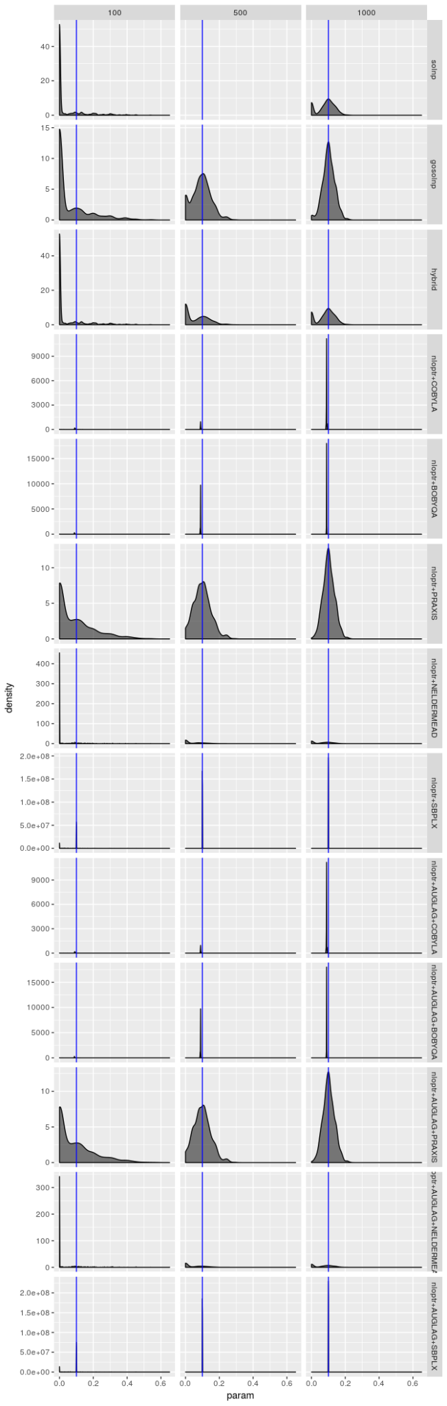
- alpha$ 估计,model 2
solver_density_plot(
    "alpha1", tags,
    list(spec2_n100, spec2_n500, spec2_n1000),
    c(100, 500, 1000), spec2)
- \(\beta\) 估计,model 2
solver_density_plot(
    "beta1", tags,
    list(spec2_n100, spec2_n500, spec2_n1000),
    c(100, 500, 1000), spec2)
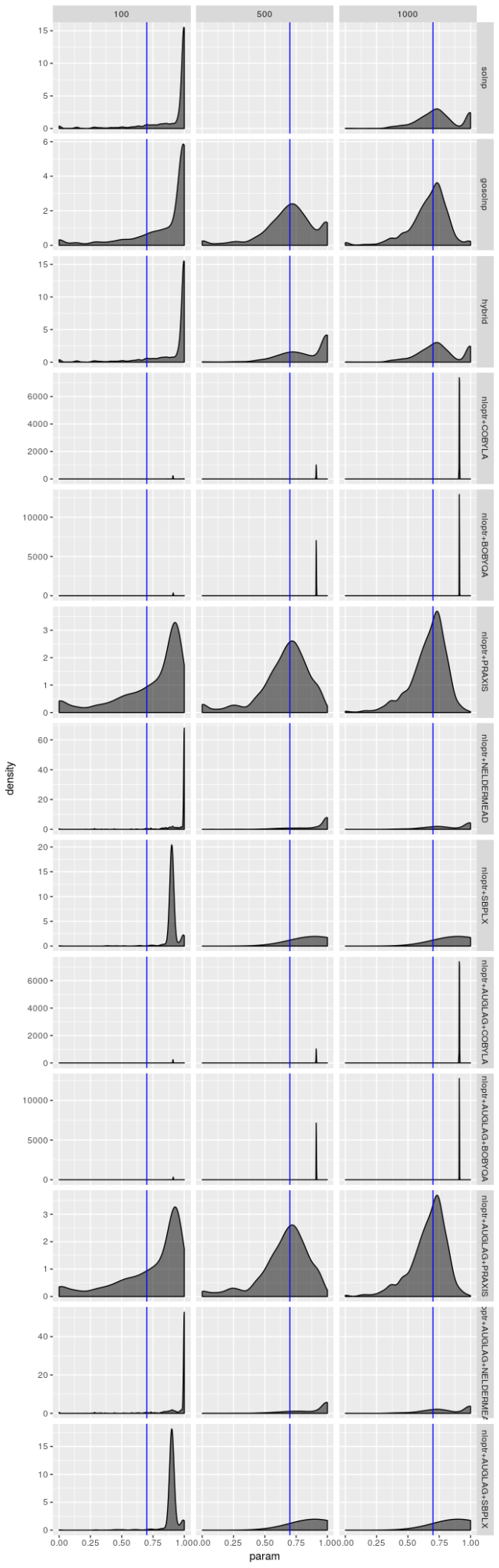
对于模型 2 来说估计器并没有那么费力,但是图显示仍然不太乐观。PRAXIS 和 AUGLAG-PRAXIS 方法似乎表现良好,但对于小样本量来说远非吸引人。
到目前为止,我的实验表明,从业者不应该依赖任何一个优化器,而是应该尝试不同的优化器,并选择具有最大对数似然的结果。假设我们将此优化算法称为“最佳”优化器。这个优化器执行效果如何?
我们来看看。
- Model 1,\(n=100\)
as.data.frame(
    round(
        solver_table(
            optMethodSims_getBestVals(
                spec1_n100, reslike = TRUE),
            "best", spec1) * 100,
        digits = 1))
##         Maximization Rate   Failure Rate   omega 95% CI Capture Rate   alpha1 95% CI Capture Rate   beta1 95% CI Capture Rate
## -----  ------------------  -------------  --------------------------  ---------------------------  --------------------------
## best                  100              0                        49.5                         63.3                        52.2
- Model 1,\(n=500\)
as.data.frame(
    round(
        solver_table(
            optMethodSims_getBestVals(
                spec1_n500, reslike = TRUE),
            "best", spec1) * 100,
        digits = 1))
##         Maximization Rate   Failure Rate   omega 95% CI Capture Rate   alpha1 95% CI Capture Rate   beta1 95% CI Capture Rate
## -----  ------------------  -------------  --------------------------  ---------------------------  --------------------------
## best                  100              0                          86                         88.8                        86.2
- Model 1,\(n=1000\)
as.data.frame(
    round(
        solver_table(
            optMethodSims_getBestVals(
                spec1_n1000, reslike = TRUE),
            "best", spec1) * 100,
        digits = 1))
##         Maximization Rate   Failure Rate   omega 95% CI Capture Rate   alpha1 95% CI Capture Rate   beta1 95% CI Capture Rate
## -----  ------------------  -------------  --------------------------  ---------------------------  --------------------------
## best                  100              0                        92.8                         90.3                        92.4
- Model 2,\(n=100\)
as.data.frame(
    round(
        solver_table(
            optMethodSims_getBestVals(
                spec2_n100, reslike = TRUE),
            "best", spec2) * 100,
        digits = 1))
##         Maximization Rate   Failure Rate   omega 95% CI Capture Rate   alpha1 95% CI Capture Rate   beta1 95% CI Capture Rate
## -----  ------------------  -------------  --------------------------  ---------------------------  --------------------------
## best                  100              0                        55.2                         63.2                        52.2
- Model 2,\(n=500\)
as.data.frame(
    round(
        solver_table(
            optMethodSims_getBestVals(
                spec2_n500, reslike = TRUE),
            "best", spec2) * 100,
        digits = 1))
##         Maximization Rate   Failure Rate   omega 95% CI Capture Rate   alpha1 95% CI Capture Rate   beta1 95% CI Capture Rate
## -----  ------------------  -------------  --------------------------  ---------------------------  --------------------------
## best                  100              0                          83                         86.3                        80.5
- Model 2,\(n=1000\)
as.data.frame(
    round(
        solver_table(
            optMethodSims_getBestVals(
                spec2_n1000, reslike = TRUE),
            "best", spec2) * 100,
        digits = 1))
##         Maximization Rate   Failure Rate   omega 95% CI Capture Rate   alpha1 95% CI Capture Rate   beta1 95% CI Capture Rate
## -----  ------------------  -------------  --------------------------  ---------------------------  --------------------------
## best                  100              0                        88.7                         91.4                        88.1
请记住,我们通过 CI 捕获率来评估“最佳”优化器的表现,该捕获率应该在 95% 左右。“最佳”优化器显然具有良好的表现,但并不优于所有优化器。这令人失望。我曾希望“最佳”优化器具有捕获率 95% 的理想特性。除了较大的样本量外,表现远不及预期。标准差被低估,或者对于小样本,正态分布很难描述估计量的实际分布(这意味着标准差乘以 2 不会导致置信区间具有所需置信水平)。
有趣的是,对于这种“最佳”估计器,两种模型之间的表现没有明显差异。这启示我,在实际数据中常见模型看似更好的结果可能正在利用优化器的偏差。
让我们看一下估计参数的分布。
- \(\omega\) 估计,model 1
solver_density_plot(
    "omega", "best",
    lapply(
        list(spec1_n100, spec1_n500, spec1_n1000),
        function(l)
        {
            optMethodSims_getBestVals(
                l, reslike = TRUE)
        }),
    c(100, 500, 1000), spec1)
- \(\alpha\) 估计,model 1
solver_density_plot(
    "alpha1", "best",
    lapply(
        list(spec1_n100, spec1_n500, spec1_n1000),
        function(l)
        {
            optMethodSims_getBestVals(
                l, reslike = TRUE)
        }),
    c(100, 500, 1000), spec1)
- \(\beta\) 估计,model 1
solver_density_plot(
    "beta1", "best",
    lapply(
        list(spec1_n100, spec1_n500, spec1_n1000),
        function(l)
        {
            optMethodSims_getBestVals(
                l, reslike = TRUE)
        }),
    c(100, 500, 1000), spec1)
- \(\omega\) 估计,model 2
solver_density_plot(
    "omega", "best",
    lapply(
        list(spec2_n100, spec2_n500, spec2_n1000),
        function(l)
        {
            optMethodSims_getBestVals(
                l, reslike = TRUE)
        }),
    c(100, 500, 1000), spec2)

- \(\alpha\) 估计,model 2
solver_density_plot(
    "alpha1", "best",
    lapply(
        list(spec2_n100, spec2_n500, spec2_n1000),
        function(l)
        {
            optMethodSims_getBestVals(
                l, reslike = TRUE)
        }),
    c(100, 500, 1000), spec2)
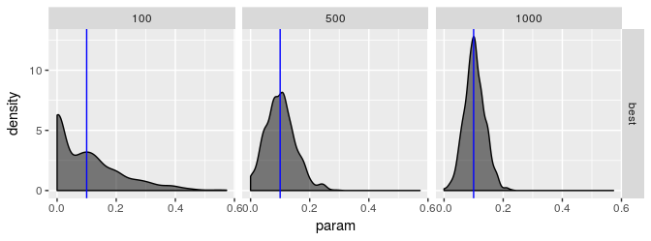
- \(\beta\) 估计,model 2
solver_density_plot(
    "beta1", "best",
    lapply(
        list(spec2_n100, spec2_n500, spec2_n1000),
        function(l)
        {
            optMethodSims_getBestVals(
                l, reslike = TRUE)
        }),
    c(100, 500, 1000), spec2)
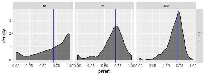
这些图表明,“最佳”估计器仍然显示出一些病态,即使它的表现不如其他估计器差。无论模型选择如何,我都没有看到参数估计有偏的证据,但我不相信“最佳”估计器真正最大化对数似然,特别是对于较小的样本量。\(\beta\) 的估计值特别糟糕。即使 \(\beta\) 的标准差应该很大,我也不认为它应该像图中揭示的那样向 0 或 1 倾斜。
结论
我最初在一年前写过这篇文章,直到现在才发表。中断的原因是因为我想得到一个关于估计 GARCH 模型参数替代方法的文献综述。不幸的是,我从未完成过这样的综述,而且我已经决定发布这篇文章。
那就是说,我会分享我正在读的东西。Gilles Zumbach 的一篇文章试图解释为什么估计 GARCH 参数很难。他指出,求解器试图最大化的准似然方程具有不良特性,例如非凸,且具有可能让算法陷入困境的“平坦”区域。他提出了另一种寻找 GARCH 模型参数的方法,在一个替代参数空间中找到最佳拟合(假设它具有比所使用 GARCH 模型的原始参数空间更好的属性),并且使用例如矩方法估计其中一个参数,而没有任何优化算法。另一篇由 Fiorentini、Calzolari 和 Panattoni 撰写的文章表明,GARCH 模型的解析梯度可以明确计算,因此这里看到的优化算法所使用的无梯度方法实际上并不是必需的。由于数值微分通常是一个难题,这可以帮助确保不会引入导致这些算法无法收敛的额外数值误差。我还想探索其他估计方法,看看它们是否能够以某种方式完全避免数值技术,或具有更好的数值属性,例如通过矩估计。我想阅读 Andersen、Chung 和 Sørensen 撰写的文章,以了解有关这种估计方法的更多信息。
然而,生活正在继续,我没有完成这篇综述。项目继续进行,基本上很好地避免了估计 GARCH 模型参数的问题。也就是说,我想重新审视这一点,或许可以探索模拟退火等技术如何用于估计 GARCH 模型参数。
所以现在,如果你是一名从业者,在估计 GARCH 模型时你应该怎么做?我想说不要理所当然地认为你的包使用的默认估计算法会起作用。你应该探索不同的算法和不同的参数选择,并使用导致最大对数似然的结果。我展示了如何以自动化方式完成这项工作,但你应该准备手动选择最佳的模型(由对数似然确定)。如果你不这样做,你估计的模型实际上可能不是理论可行的模型。
我将在本文的最后再次说一遍,特别强调:不要将数值技术和结果视为理所当然的!
sessionInfo()
## R version 3.4.2 (2017-09-28)
## Platform: i686-pc-linux-gnu (32-bit)
## Running under: Ubuntu 16.04.2 LTS
##
## Matrix products: default
## BLAS: /usr/lib/libblas/libblas.so.3.6.0
## LAPACK: /usr/lib/lapack/liblapack.so.3.6.0
##
## locale:
##  [1] LC_CTYPE=en_US.UTF-8       LC_NUMERIC=C
##  [3] LC_TIME=en_US.UTF-8        LC_COLLATE=en_US.UTF-8
##  [5] LC_MONETARY=en_US.UTF-8    LC_MESSAGES=en_US.UTF-8
##  [7] LC_PAPER=en_US.UTF-8       LC_NAME=C
##  [9] LC_ADDRESS=C               LC_TELEPHONE=C
## [11] LC_MEASUREMENT=en_US.UTF-8 LC_IDENTIFICATION=C
##
## attached base packages:
## [1] parallel  stats     graphics  grDevices utils     datasets  methods
## [8] base
##
## other attached packages:
## [1] ggplot2_2.2.1 rugarch_1.3-8 printr_0.1
##
## loaded via a namespace (and not attached):
##  [1] digest_0.6.16               htmltools_0.3.6
##  [3] SkewHyperbolic_0.3-2        expm_0.999-2
##  [5] scales_0.5.0                DistributionUtils_0.5-1
##  [7] Rsolnp_1.16                 rprojroot_1.2
##  [9] grid_3.4.2                  stringr_1.3.1
## [11] knitr_1.17                  numDeriv_2016.8-1
## [13] GeneralizedHyperbolic_0.8-1 munsell_0.4.3
## [15] pillar_1.3.0                tibble_1.4.2
## [17] compiler_3.4.2              highr_0.6
## [19] lattice_0.20-35             labeling_0.3
## [21] Matrix_1.2-8                KernSmooth_2.23-15
## [23] plyr_1.8.4                  xts_0.10-0
## [25] spd_2.0-1                   zoo_1.8-0
## [27] stringi_1.2.4               magrittr_1.5
## [29] reshape2_1.4.2              rlang_0.2.2
## [31] rmarkdown_1.7               evaluate_0.10.1
## [33] gtable_0.2.0                colorspace_1.3-2
## [35] yaml_2.1.14                 tools_3.4.2
## [37] mclust_5.4.1                mvtnorm_1.0-6
## [39] truncnorm_1.0-7             ks_1.11.3
## [41] nloptr_1.0.4                lazyeval_0.2.1
## [43] crayon_1.3.4                backports_1.1.1
## [45] Rcpp_1.0.0

 浙公网安备 33010602011771号