Amber TUTORIAL B1: Simulating a DNA polyA-polyT Decamer

Section 1: Introduction

The input files required (using their default file names):

• prmtop - a file containing a description of the molecular topology and the necessary force field parameters.
• inpcrd (or a restrt from a previous run) - a file containing a description of the atom coordinates and optionally velocities and current periodic box dimensions.
• mdin - the sander input file consisting of a series of namelists and control variables that determine the options and type of simulation to be run.

The approximate order of this tutorial will be as follows:

1. Create the prmtop and inpcrd files: This is a description of how to generate the initial structure and set up the molecular topology/parameter and coordinate files necessary for performing minimization or dynamics with sander.
2. An introduction to minimization and molecular dynamics. Run short MD simulations in-vacuo. Perform basic analysis such as calculating root-mean-squared deviations (RMSd) and plotting various energy terms as a function of time. Visualizing results with VMD.
3. Minimization and molecular dynamics in implicit solvent: Setting up and running equilibration and production minimization and molecular dynamics simulations for our DNA model using the Born implicit solvent model.
4. Minimization and molecular dynamics in explicit solvent: Setting up and running equilibration and production simulations for our DNA model using TIP3P explicit water.

Section 2: Setting up duplex DNA: polyA-polyT

2.1) Generating the coordinates of the model structure

2.1.1) Creating our DNA duplex using NAB

构建NAB输入文件nuc.nab

$$$ nuc.nab

molecule m; 
m = fd_helix( "abdna", "aaaaaaaaaa", "dna" );
putpdb( "nuc.pdb", m, "-wwpdb");

Running NAB

nab nuc.nab
./a.out (Note: type "./a.exe" for  Cygwin/Windows)

2.1.2) Loading the structure into Leap

以下命令可以分步再xleap中或tleap中运行，也可把下列命令放到名为 tleap.in 的文件中，用命令 tleap -f tleap.in 执行，下面命令会产生三种不同的模型，详情看注释内容

source leaprc.DNA.bsc1
source leaprc.water.tip3p
dna1= loadpdb "nuc.pdb"

# An in vacuo model of the poly(A)-poly(T) structure (named polyAT_vac)
saveamberparm dna1 polyAT_vac.prmtop polyAT_vac.inpcrd

# An in vacuo model of the poly(A)-poly(T) structure with explicit counterions (named polyAT_cio)
addions dna1 Na+ 0
saveamberparm dna1 polyAT_cio.prmtop polyAT_cio.inpcrd

# A TIP3P (water) solvated model of the poly(A)-poly(T) structure in a periodic box (named polyAT_wat)
dna2 = copy dna1
solvatebox dna1 TIP3PBOX 8.0
solvateoct dna2 TIP3PBOX 8.0
saveamberparm dna2 polyAT_wat.prmtop polyAT_wat.inpcrd

quit

其中，可以运行以下命令增加对leap的理解：

edit dna1　　　　　　　　　　　　# 可在xleap状态下查看目标结构
help loadpdb　　　　　　　　　　# loadpdb帮助文档
help saveamberparm
help addions
help solvatebox
help solvateoct
list　　　　　　　　　　　　　　# 列举当前力场下载入的所有原子，分子，离子及水模型

Section 3: Running Minimization and Molecular Dynamics (in vacuo)

This section of the tutorial will consist of 3 stages:

1. Relaxing the system prior to MD
2. Molecular dynamics at constant temperature
3. Analyzing the results

3.1) Relaxing the System Prior to MD

The basic usage for sander is as follows:

sander [-O] -i mdin -o mdout -p prmtop -c inpcrd -r restrt [-ref refc] [-x mdcrd] [-v mdvel] [-e mden] [-inf mdinfo]

• Arguments in []'s are optional
• If an argument is not specified, the default name will be used.
• -O    overwrite all output files (the default behavior is to quit if any output files already exist)
• -i      the name of the input file (which describes the simulation options), mdin by default.
• -o     the name of the output file, mdout by default.
• -p     the parameter/topology file, prmtop by default.
• -c     the set of initial coordinates for this run, inpcrd by default.
• -r     the final set of coordinates from this MD or minimization run, restrt by default.
• -ref  reference coordinates for positional restraints, if this option is specified in the input file, refc by default.
• -x    the molecular dynamics trajectory file (if running MD), mdcrd by default.
• -v    the molecular dynamics velocities file (if running MD), mdvel by default.
• -e    a summary file of the energies (if running MD), mden by default.
• -inf  a summary file written every time energy information is printed in the output file for the current step of the minimization of MD, useful for checking on the progress of a simulation, mdinfo by default.

3.1.1) Building the mdin input file

因为先前步骤产生的默认结构并不是能量最优的，内部可能存在原子间的conflict和overlap，这可能使MD模拟变得不稳定，所以最好再MD之前先对初始结构进行优化(minimization)

$$$   polyAT_vac_init_min.in

polyA-polyT 10-mer: initial minimization prior to MD
 &cntrl
  imin   = 1,
  maxcyc = 500,
  ncyc   = 250,
  ntb    = 0,
  igb    = 0,
  cut    = 12
 /

上面为指定sander输入的namelist 变量文件，除最开始的说明信息外，此文件通常以&cntrl或&ewald开头，以“/”结尾，下面一段英文是对polyAT_vac_init_min.in文件的论述；

　　To turn on minimization, we specify IMIN = 1. We want a fairly short minimization since we don't actually need to reach the minima, but just want to move away from any local maxima, so we select 500 steps of minimization by specifying MAXCYC = 500. Sandersupports a number of different minimization algorithms, the most commonly used being steepest descent and conjugate gradient. The steepest descent algorithm is good for quickly removing the largest strains in the system but it also converges slowly when close to a minima. Here the conjugate gradient method is more efficient. The use of these two algorithms can be controlled using the NCYC flag. If NCYC < MAXCYC, sander will use the steepest descent algorithm for the first NCYC steps before switching to the conjugate gradient algorithm for the remaining (MAXCYC - NCYC) steps. In this case we will run an equal number of steps with each algorithm so we set NCYC = 250. Since sander assumes that the system is periodic by default we need to explicitly turn this off (NTB = 0). In this simulation we will be using a constant dielectric and not an implicit (or explicit) solvent model so we set IGB = 0 (no generalized born solvation model). This is the default so we  don't strictly need to specify this, but I will include it here so that we can see what differences we have in the input file when we switch on implicit solvent later. We also need to choose a value for the non-bonded cut off. A larger cut off introduces less error in the non-bonded force evaluation but increases the computational complexity and thus calculation time. 12 angstroms would seem like a reasonable tradeoff for gas phase so that is what we will initially use (CUT = 12).

3.1.2) Running sander for the first time

指定好namelist文件后，执行sander：

sander -O -i polyAT_vac_init_min.in -o polyAT_vac_init_min.out -c polyAT_vac.inpcrd -p polyAT_vac.prmtop -r polyAT_vac_init_min.rst

Input files: polyAT_vac_init_min.in, polyAT_vac.inpcrd, polyAT_vac.prmtop
Output files: polyAT_vac_init_min.out, polyAT_vac_init_min.rst

3.1.3) Creating PDB files from the AMBER coordinate files

使用ambpdb命令可以从rst文件中提取pdb信息：

ambpdb -p polyAT_vac.prmtop -c polyAT_vac_init_min.rst > polyAT_vac_init_min.pdb

3.2) Running MD in-vacuo (100ps)

通过比较两种不同的cut值，我们可以更加明确cut的意义：

$$$ polyAT_vac_md1_12Acut.in

10-mer DNA MD in-vacuo, 12 angstrom cut off
 &cntrl
  imin = 0, ntb = 0,
  igb = 0, ntpr = 100, ntwx = 100,
  ntt = 3, gamma_ln = 1.0,
  tempi = 300.0, temp0 = 300.0
  nstlim = 100000, dt = 0.001,
  cut = 12.0
 /

 

$$$ polyAT_vac_md1_nocut.in

10-mer DNA MD in-vacuo, infinite cut off
 &cntrl
  imin = 0, ntb = 0,
  igb = 0, ntpr = 100, ntwx = 100,
  ntt = 3, gamma_ln = 1.0,
  tempi = 300.0, temp0 = 300.0
  nstlim = 100000, dt = 0.001,
  cut = 999
 /

 To run a molecular dynamics simulation with sander, we need to turn off minimization (IMIN=0). Since we are running in-vacuo we also need to disable periodicity (NTB=0) and set IGB=0 since we are not using implicit solvent. For these two examples we will write information to the output file and trajectory coordinates file every 100 steps (NTPR=100, NTWX=100). The CUT variable specifies the cut off range for the long range non-bonded interactions. Here, two different values for the cutoff will be used, one run with a cut off of 12 angstroms (CUT = 12.0) and one run without a cutoff. To run without a cutoff we simply set CUT to be larger than the extent of the system (e.g. CUT = 999). For temperature regulation we will use the Langevin thermostat (NTT=3) to maintain the temperature of our system at 300 K. This temperature control method uses Langevin dynamics with a collision frequency given by GAMMA_LN and is significantly more efficient at equilibrating the system temperature than the Berendsen temperature coupling scheme (NTT=1). For simplicity we will run this entire simulation with NTT=3 and GAMMA_LN=1. We shall also set the initial and final temperatures to 300 K (TEMPI=300.0, TEMP0=300.0) which will mean our system's temperature should remain around 300 K. In these two examples we will run a total of 100,000 steps each (NSTLIM=100000) with a 1 fs time step (DT=0.001) giving simulation lengths of 100 ps (100,000 x 1fs).

运行真空状态下MD（也可用sander.MP或pmemd或pmemd.MPI）：

CUT=12.0:

sander -O -i polyAT_vac_md1_12Acut.in -o polyAT_vac_md1_12Acut.out -c polyAT_vac_init_min.rst -p polyAT_vac.prmtop -r polyAT_vac_md1_12Acut.rst -x polyAT_vac_md1_12Acut.mdcrd

CUT=999:

sander -O -i polyAT_vac_md1_nocut.in -o polyAT_vac_md1_nocut.out -c polyAT_vac_init_min.rst -p polyAT_vac.prmtop -r polyAT_vac_md1_nocut.rst -x polyAT_vac_md1_nocut.mdcrd

实时观测程序输出：

tail -f polyAT_vac_md1_12Acut.out

3.3) Analyzing the results

3.3.1) Extracting the energies, etc. from the mdout file

使用process_mdout.perl脚本，从mdout文件中提取能量势能等信息：

mkdir polyAT_vac_md1_12Acut
cd polyAT_vac_md1_12Acut
process_mdout.perl ../polyAT_vac_md1_12Acut.out

 

mkdir polyAT_vac_md1_nocut
cd polyAT_vac_md1_nocut
process_mdout.perl ../polyAT_vac_md1_nocut.out

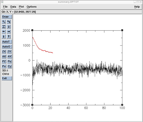
用grace对各个能量进行绘图：

xmgrace ./polyAT_vac_md1_12Acut/summary.EPTOT ./polyAT_vac_md1_nocut/summary.EPTOT

 图表如下：

 

3.3.2) Calculating the RMSd vs. time

计算12Acut RMSD变化情况：

trajin polyAT_vac_md1_12Acut.mdcrd
rms first mass out polyAT_vac_md1_12Acut.rms time 0.1

计算nocut RMSD变化情况：

trajin polyAT_vac_md1_nocut.mdcrd
rms first mass out polyAT_vac_md1_nocut.rms time 0.1

where trajin specifies the name of the trajectory file to process, rms first mass tells cpptraj that we want it to calculate a MASS weighted, RMS fit to the FIRST structure. out specifies the name of the file to write the results to and time 0.1 tells cpptraj that each frame of the coordinate file represents 0.1 ps. Since we have two simulations we have two input files, with different trajectory and output files in each.

使用cpptraj程序：

$AMBERHOME/bin/cpptraj -p polyAT_vac.prmtop -i polyAT_vac_md1_12Acut.calc_rms
$AMBERHOME/bin/cpptraj -p polyAT_vac.prmtop -i polyAT_vac_md1_nocut.calc_rms

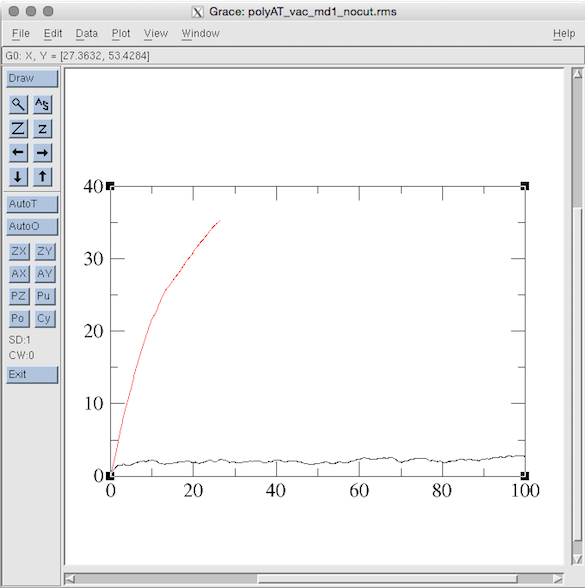
使用grace作图：

>xmgrace polyAT_vac_md1_12Acut.rms polyAT_vac_md1_nocut.rms

 图表如下：

 

Section 4: Running Minimization and MD (in implicit solvent)

与第三节相同的是，在正式做MD之前需要对体系进行优化，不同的是，这节的运行环境不再是真空(vacuo)，而是在隐式溶剂模型中(implicit solvent model)，这种模型相对于真空更加与真实环境相近，同时运算量也要大很多，效果比真空环境好，但是不如准确溶剂模型(explicit solvent model)，但是explicit solvent计算资源耗费更大。

Use of the Born solvation model is controlled by the IGB flag. The default value for this flag is 0 which corresponds to no generalized Born term being used. Alternative values are IGB=1 which corresponds to the "standard" pairwise generalized Born model using the default radii set up by LEaP (the method we will be using here), IGB=2 a modified GB model developed by A. Onufriev, D. Bashford and D.A.Case and IGB=5 which is essentially the same as IGB=2 but with alternative parameters. For further details see the AMBER manual.

4.1) Relaxing the System Prior to MD

generalized Born method (IGB=1), CUT=12.0

$$$ polyAT_gb_init_min.in

polyA-polyT 10-mer: initial minimization prior to MD GB model
 &cntrl
  imin   = 1,
  maxcyc = 500,
  ncyc   = 250,
  ntb    = 0,
  igb    = 1,
  cut    = 12
 /

运行sander(也可使用pmemd):

sander -O -i polyAT_gb_init_min.in -o polyAT_gb_init_min.out -c polyAT_vac.inpcrd -p polyAT_vac.prmtop -r polyAT_gb_init_min.rst

分析优化后pdb结构：

ambpdb -p polyAT_vac.prmtop -c polyAT_gb_init_min.rst > polyAT_gb_init_min.pdb

4.2) Running MD with generalized Born solvation

$$$   polyAT_gb_md1_12Acut.in　　　　　　　　　　　　　　# 12.0 angstrom long range cutoff, Generalized Born

10-mer DNA MD Generalized Born, 12 angstrom cut off
 &cntrl
  imin = 0, ntb = 0,
  igb = 1, ntpr = 100, ntwx = 100,
  ntt = 3, gamma_ln = 1.0,
  tempi = 300.0, temp0 = 300.0
  nstlim = 100000, dt = 0.001,
  cut = 12.0
 /

 

$$$ polyAT_gb_md1_nocut.in　　　　　　　　　　　　　　# no long range cutoff, Generalized Born

10-mer DNA MD Generalized Born, infinite cut off
 &cntrl
  imin = 0, ntb = 0,
  igb = 1, ntpr = 100, ntwx = 100,
  ntt = 3, gamma_ln = 1.0,
  tempi = 300.0, temp0 = 300.0
  nstlim = 100000, dt = 0.001,
  cut = 999
 /

We are using the same settings as before, namely we turn off minimization (IMIN=0). We disable periodicity (NTB=0) but this time set IGB=1 since we want to use the Born implicit solvent model. We will again write information to the output file and trajectory coordinates file every 100 steps (NTPR=100, NTWX=100). Two different values for the cutoff will be used, one run will be with a cutoff of 12 angstroms (CUT = 12.0) and one run will be without a cutoff (CUT = 999). For temperature regulation we will use the Langevin thermostat (NTT=3, GAMMA_LN=1) to maintain the temperature of our system at 300 K.

We shall also set the initial and final temperatures to 300 K (TEMPI=300.0, TEMP0=300.0) which will mean our system's temperature should remain around 300 K. Again we will run the two examples for a total of 100,000 steps each (NSTLIM=100000) with a 1 fs time step (DT=0.001) giving simulation lengths of 100 ps (100,000 x 1fs).

As mentioned in the previous section when running production simulations with ntt=2 or 3 you should always change the random seed (ig) between restarts. You can achieve this automatically by setting ig=-1 in the ctrl namelist. We do not do this here in the tutorial for reproducibility but it is generally recommended that you do this in your calculations. 

 

运行100ns MD（也可用sander.MP或pmemd或pmemd.MPI）：

sander -O -i polyAT_gb_md1_12Acut.in -o polyAT_gb_md1_12Acut.out -c polyAT_gb_init_min.rst -p polyAT_vac.prmtop -r polyAT_gb_md1_12Acut.rst -x polyAT_gb_md1_12Acut.mdcrd

 

sander -O -i polyAT_gb_md1_nocut.in -o polyAT_gb_md1_nocut.out -c polyAT_gb_init_min.rst -p polyAT_vac.prmtop -r polyAT_gb_md1_nocut.rst -x polyAT_gb_md1_nocut.mdcrd

实时观测程序输出：

tail -f polyAT_gb_md1_12Acut.out

4.3) Analyzing the results

使用process_mdout.perl脚本，从mdout文件中提取能量势能等信息：

mkdir polyAT_gb_md1_12Acut
mkdir polyAT_gb_md1_nocut
cd polyAT_gb_md1_12Acut
process_mdout.perl ../polyAT_gb_md1_12Acut.out
cd ../polyAT_gb_md1_nocut
process_mdout.perl ../polyAT_gb_md1_nocut.out
cd ..
xmgrace ./polyAT_gb_md1_12Acut/summary.EPTOT ./polyAT_gb_md1_nocut/summary.EPTOT

结果如图:

计算RMSD变化情况：

$$$ polyAT_gb_md1_12Acut.calc_rms

trajin polyAT_gb_md1_12Acut.mdcrd
rms first mass out polyAT_gb_md1_12Acut.rms time 0.1

 

$$$ polyAT_gb_md1_nocut.calc_rms

trajin polyAT_gb_md1_nocut.mdcrd
rms first mass out polyAT_gb_md1_nocut.rms time 0.1

 使用cpptraj分析RMSD变化：

$AMBERHOME/bin/cpptraj -p polyAT_vac.prmtop -i polyAT_gb_md1_12Acut.calc_rms 
$AMBERHOME/bin/cpptraj -p polyAT_vac.prmtop -i polyAT_gb_md1_nocut.calc_rms
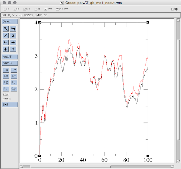
xmgrace polyAT_gb_md1_12Acut.rms polyAT_gb_md1_nocut.rms

 grace作图：

 

Section 5: Running Minimization and MD (in explicit solvent)

5.1) Equilibrating and running MD with solvated poly(A)-poly(T)

因为准确溶剂化模型的原因，此次对模型的优化分为两个阶段，第一阶段保持溶质固定，优化溶剂及离子；第二阶段优化整个体系：

5.1.1) Minimization Stage 1 - Holding the solute fixed

$$$ polyAT_wat_min1.in

polyA-polyT 10-mer: initial minimization solvent + ions
 &cntrl
  imin   = 1,
  maxcyc = 1000,
  ncyc   = 500,
  ntb    = 1,
  ntr    = 1,
  cut    = 10.0
 /
Hold the DNA fixed
500.0
RES 1 20
END
END

The meaning of each of the terms are as follows:

• IMIN = 1: Minimization is turned on (no MD)
• MAXCYC = 1000: Conduct a total of 1,000 steps of minimization.
• NCYC = 500: Initially do 500 steps of steepest descent minimization followed by 500 steps (MAXCYC - NCYC) steps of conjugate gradient minimization.
• NTB = 1: Use constant volume periodic boundaries (PME is always "on" when NTB > 0).
• CUT = 10.0: Use a cutoff of 10 angstroms. (This is probably overkill here, we could get away with 8.0 or 9.0 angstroms if we wanted but using a larger cutoff does not harm the accuracy of the results. It just makes the calculations slightly more costly.)
• NTR = 1: Use position restraints based on the GROUP input given in the input file. GROUP input is described in detail in the appendix of the user's manual. In this example, we use a force constant of 500 kcal mol^-1 angstrom^-2 and restrain residues 1 through 20 (the DNA). This means that the water and counterions are free to move. The GROUP input is the last 5 lines of the input file:

• Hold the DNA fixed
  500.0
  RES 1 20
  END
  END

  Note that whenever you run using the GROUP option in the input you should carefully check the top of the output file to make sure you've selected as many atoms as you thought you did. (Note also that 500 kcal/mol-A**2 is a very large force constant, much larger than is needed. You can use this for minimization, but for dynamics, stick to much smaller values, say around 10.)

运行sander(pmemd)进行第一阶段优化：

sander -O -i polyAT_wat_min1.in -o polyAT_wat_min1.out -p polyAT_wat.prmtop -c polyAT_wat.inpcrd -r polyAT_wat_min1.rst -ref polyAT_wat.inpcrd

5.1.2) Minimization Stage 2 - Minimizing the entire system

$$$ polyAT_wat_min2.in

polyA-polyT 10-mer: initial minimization whole system
 &cntrl
  imin   = 1,
  maxcyc = 2500,
  ncyc   = 1000,
  ntb    = 1,
  ntr    = 0,
  cut    = 10.0
 /

运行sander(pmemd)进行第二阶段优化：

sander -O -i polyAT_wat_min2.in -o polyAT_wat_min2.out -p polyAT_wat.prmtop -c polyAT_wat_min1.rst -r polyAT_wat_min2.rst

提出pdb，查看结构差别：

$AMBERHOME/bin/ambpdb -p polyAT_wat.prmtop < polyAT_wat.inpcrd > polyAT_wat.pdb

$AMBERHOME/bin/ambpdb -p polyAT_wat.prmtop < polyAT_wat_min2.rst > polyAT_wat_min2.pdb

注：ambpdb出现Error: Could not read restart atoms/time.时，命令变更为 ambpdb -p polyAT_wat.prmtop -c polyAT_wat_min2.rst > polyAT_wat_min2.pdb .

5.1.3) Molecular Dynamics (heating) with restraints on the solute

$$$ polyAT_wat_md1.in

polyA-polyT 10-mer: 20ps MD with res on DNA
 &cntrl
  imin   = 0,
  irest  = 0,
  ntx    = 1,
  ntb    = 1,
  cut    = 10.0,
  ntr    = 1,
  ntc    = 2,
  ntf    = 2,
  tempi  = 0.0,
  temp0  = 300.0,
  ntt    = 3,
  gamma_ln = 1.0,
  nstlim = 10000, dt = 0.002
  ntpr = 100, ntwx = 100, ntwr = 1000
 /
Keep DNA fixed with weak restraints
10.0
RES 1 20
END
END

As mentioned in Section 3, when running production simulations with ntt=2/3 you should always change the random seed (ig) between restarts. If you are using AMBER 10 (bugfix.26 or later) or AMBER 11 or later then you can achieve this automatically by setting ig=-1 in the ctrl namelist. We do not do this here in the tutorial for reproducibility but it is generally recommended that you do this in your calculations.

The meaning of each of the terms are as follows:

• IMIN = 0: Minimization is turned off (run molecular dynamics)
• IREST = 0, NTX = 1: We are generating random initial velocities from a Boltzmann distribution and only read in the coordinates from the inpcrd. In other words, this is the first stage of our molecular dynamics. Later we will change these values to indicate that we want to restart a molecular dynamics run from where we left off.
• NTB = 1: Use constant volume periodic boundaries (PME is always "on" when NTB>0).
• CUT = 10.0: Use a cutoff of 10 angstroms.
• NTR = 1: Use position restraints based on the GROUP input given in the input file. In this case we will restrain the DNA with a force constant of 10 angstroms.
• NTC = 2, NTF = 2: SHAKE should be turned on and used to constrain bonds involving hydrogen.
• TEMPI = 0.0, TEMP0 = 300.0: We will start our simulation with a temperature, derived from the kinetic energy, of 0 K and we will allow it to heat up to 300 K. The system should be maintained, by adjusting the kinetic energy, as 300 K.
• NTT = 3, GAMMA_LN = 1.0: The Langevin dynamics should be used to control the temperature using a collision frequency of 1.0 ps^-1.
• NSTLIM = 10000, DT = 0.002: We are going to run a total of 10,000 molecular dynamics steps with a time step of 2 fs per step, possible since we are now using SHAKE, to give a total simulation time of 20 ps.
• NTPR = 100, NTWX = 100, NTWR = 1000: Write to the output file (NTPR) every 100 steps (200 fs), to the trajectory file (NTWX) every 100 steps and write a restart file (NTWR), in case our job crashes and we want to restart it, every 1,000 steps.

 运行sander(pmemd, pmemd.MPI etc.)进行限制性pre-MD (heating):

sander -O -i polyAT_wat_md1.in -o polyAT_wat_md1.out -p polyAT_wat.prmtop -c polyAT_wat_min2.rst -r polyAT_wat_md1.rst -x polyAT_wat_md1.mdcrd -ref polyAT_wat_min2.rst

 

5.1.6) Running MD Equilibration on the whole system

$$$ polyAT_wat_md2.in

polyA-polyT 10-mer: 100ps MD
 &cntrl
  imin = 0, irest = 1, ntx = 7,
  ntb = 2, pres0 = 1.0, ntp = 1,
  taup = 2.0,
  cut = 10.0, ntr = 0,
  ntc = 2, ntf = 2,
  tempi = 300.0, temp0 = 300.0,
  ntt = 3, gamma_ln = 1.0,
  nstlim = 50000, dt = 0.002,
  ntpr = 100, ntwx = 100, ntwr = 1000
 /

The meaning of each of the terms are as follows:

• IMIN = 0: Minimization is turned off (run molecular dynamics)
• IREST = 1, NTX = 7: We want to restart our MD simulation where we left off after the 20 ps of constant volume simulation. IREST tells sander that we want to restart a simulation, so the time is not reset to zero but will start at 20 ps. Previously we have had NTX set at the default of 1 which meant only the coordinates were read from the restrt file. This time, however, we want to continue from where we finished so we set NTX = 7 which means the coordinates, velocities and box information will be read from a formatted (ASCII) restrt file.
• NTB = 2, PRES0 = 1.0, NTP = 1, TAUP = 2.0: Use constant pressure periodic boundary with an average pressure of 1 atm (PRES0). Isotropic position scaling should be used to maintain the pressure (NTP=1) and a relaxation time of 2 ps should be used (TAUP=2.0).
• CUT = 10.0: Use a cut off of 10 angstroms.
• NTR = 0: We are no longer using positional restraints.
• NTC = 2, NTF = 2: SHAKE should be turned on and used to constrain bonds involving hydrogen.
• TEMPI = 300.0, TEMP0 = 300.0: Our system was already heated to 300 K during the first stage of MD so here it will start at 300 K and should be maintained at 300 K.
• NTT = 3, GAMMA_LN = 1.0: The Langevin dynamics should be used to control the temperature using a collision frequency of 1.0 ps^-1.
• NSTLIM = 50000, DT = 0.002: We are going to run a total of 50,000 molecular dynamics steps with a time step of 2 fs per step, possible since we are now using SHAKE, to give a total simulation time of 100 ps.
• NTPR = 100, NTWX = 100, NTWR = 1000: Write to the output file (NTPR) every 100 steps (200 fs), to the trajectory file (NTWX) every 100 steps and write a restart file (NTWR), in case our job crashes and we want to restart it, every 1,000 steps.

 对整个体系进行MD running (sander, sander.MPI, pmemd, pmemd.MPI)

sander -O -i polyAT_wat_md2.in -o polyAT_wat_md2.out -p polyAT_wat.prmtop -c polyAT_wat_md1.rst -r polyAT_wat_md2.rst -x polyAT_wat_md2.mdcrd

 

5.2) Analyzing the results to test the equilibration

5.2.1) Analyzing the output files

mkdir analysis
cd analysis
process_mdout.perl ../polyAT_wat_md1.out ../polyAT_wat_md2.out
xmgrace summary.EPTOT summary.EKTOT summary.ETOT
xmgrace summary.TEMP
xmgrace summary.PRES

 

vi summary.VOLUME
d100    (removes the current (first) line plus the next 100 lines)
<esc>:wq summary.VOLUME.modified

xmgrace summary.VOLUME.modified

5.2.2) Analyzing the trajectory

trajin polyAT_wat_md1.mdcrd
trajin polyAT_wat_md2.mdcrd
rms first out polyAT_wat_backbone.rms @P,O3',O5',C3',C4',C5' time 0.2

$AMBERHOME/bin/cpptraj -p polyAT_wat.prmtop -i polyAT_wat_calc_backbone_rms.in

xmgrace polyAT_wat_backbone.rms