R语言实现多组样本两两t检验的完整教程

t检验的核心思想是通过样本均值与方差的比较，评估两个总体均值是否存在显著差异。当有三个或更多组数据时，单次t检验已不再适用，因此通常的做法是先进行方差齐性检验与单因素方差分析（ANOVA），如果总体差异显著，再进行组间的两两t检验，用于具体比较每对样本组之间的差异。

多组样本执行两两t.test时，当有分组少于2个数据，t.test会报错，当要检测的数据为常量时，t.test会报错，

下面代码将解决以上问题

library(readr)
library(dplyr)
library(purrr)
library(rstatix)
# 构建函数进行两两t.test
pf_ttest <- function(my_comparison, data) {
  group1 <- my_comparison[1]
  group2 <- my_comparison[2]

  data1 <- filter(data, group == group1) %>% pull(value)
  data2 <- filter(data, group == group2) %>% pull(value)

  cat(sprintf("比较 %s (n=%d) vs %s (n=%d)\n", group1, length(data1), group2, length(data2)))

  tryCatch(
    {
      test_result <- t.test(data1, data2)
      tibble(
        group1 = group1,
        group2 = group2,
        p = test_result$p.value,
        statistic = test_result$statistic,
        df = test_result$parameter
      )
    },
    error = function(e) {
      cat(sprintf("错误: %s\n", e$message))
    }
  )
}

# 创建比较组
create_comparisons <- function(groups) {
  comp <- combn(groups, 2)
  lapply(1:ncol(comp), function(i) as.character(comp[, i]))
}


# 准备数据：2列，第1列为分组，第2列为数值
data <- readxl::read_xlsx("OP.xlsx")
col_names <- names(data)
xlab=col_names[1]
ylab=col_names[2]
data=dplyr::rename(data, group = 1, value = 2)

# 创建比较组
my_comparisons <- create_comparisons(unique(data$group))

stat_test <- map_dfr(my_comparisons, pf_ttest, data) %>%
  mutate(p.adj = p.adjust(p)) %>%
  add_significance(
    p.col = "p.adj",
    cutpoints = c(0, 0.001, 0.01, 0.05, 1),
    symbols = c("***", "**", "*", "ns")
  )

比较 Homo sapiens (n=22) vs M. assmensiss (n=4)

比较 Homo sapiens (n=22) vs M.mulatta (n=1)

错误: 'y'观察值数量不足

比较 Homo sapiens (n=22) vs M. arctoides (n=2)

比较 Homo sapiens (n=22) vs M. mulatta (n=15)

比较 Homo sapiens (n=22) vs M. fascicularis (n=1)

错误: 'y'观察值数量不足

比较 0mascus leucogenys (n=25) vs Pongo pygmaeus (n=7)

head(stat_test)

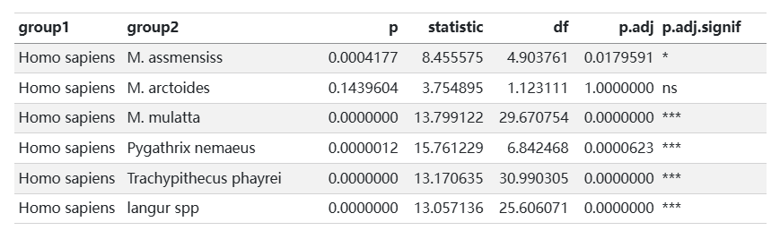
write_tsv(stat_test, "stat_test.tsv")

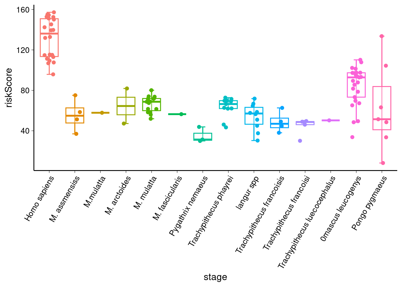
# 绘制箱形图
sig_comparisons <- stat_test %>%
  filter(p < 0.05) %>%
  select(group1, group2) %>%
  as.data.frame() %>% # 确保是 data.frame
  split(1:nrow(.)) %>% # 按行分割
  lapply(function(x) as.character(x))


# 创建基础图形
library(ggpubr)
p1 <- ggboxplot(data,
  x = "group",
  y = "value",
  color = "group",
  alpha = 0.3,
  xlab = xlab,
  ylab = ylab,
  bxp.errorbar = TRUE,
  bxp.errorbar.width = 0.2,
  add = "jitter",
  legend = "none"
) +
  theme(
    plot.title = element_text(size = 15, hjust = 0.5),
    axis.title = element_text(size = 12),
    axis.text.x = element_text(size = 10, angle = 60, hjust = 1),
    axis.text.y = element_text(size = 10),
    axis.ticks = element_line(linewidth = 0.2),
  )

p1

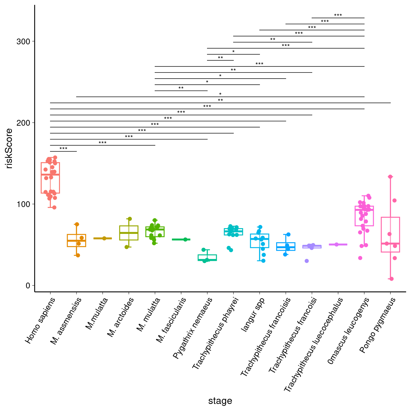
p1 + stat_compare_means(
    comparisons = sig_comparisons,
    method = "t.test",
    label = "p.signif", # 显示显著性符号（*, **, ***）
    symnum.args = list(
      cutpoints = c(0, 0.001, 0.01, 0.05, Inf),
      symbols = c("***", "**", "*", "ns")
    ),
    hide.ns = TRUE, # 隐藏不显著的标签
    vjust = 0.75,
    tip.length = 0,
    step.increase = 0.05,
    size = 3
  )