Tree - AdaBoost with sklearn source code
In the previous post we addressed some issue of decision tree, including instability, lack of smoothness, sensitivity to data, and etc.
One solution is Boosting Method. In simple words Boosting combines multiple weak learners to get a powerful prediction, where the weak learner are usually shallow tree.
Before we go to the popularly used boosting algorithm like GBM(GBRT) and xgBoost, let's start with one of the earliest Boosting Method - AdaBoost.
AdaBoost Evolution
Early AdaBoost focus on binary classification only. And then it extend to regression problem and multi-class classification. Let's go through them one by one.
Discrete AdaBoost (Freund & Schapire 1996)
A concise description of Discrete AdaBoost is that at each step a base binary classifier (\(f_m(x) \in \{-1,1 \}\)) is trained against a weighted training sample. The weight of misclassified sample will increase, and then another classifier will be trained with updated weight. The final result will be a weighted sum of all base classifiers.
- assign equal weight to all sample \(w_i = 1/N\)
- Repeat below m times
A. Fit classifier \(f_m(x) \in \{-1,1\}\), by minimizing a weighted loss function
B. Compute weighted misclassification rate \(e_m = E_w[I(y\ne f_m(x))] = \sum_i{w_i \cdot I(y\ne f_m(x)) }\)
C. Compute classifier weight \(c_m = log((1-e_m)/e_m)\)
D. Update sample weight \(w_i = w_i * exp(c_m \cdot I(y\ne f_m(x))\)
E. Normalize weight so that \(\sum_i{w_i} = 1\)
- Output the classifier \(sign[\sum_{i=1}^M c_m f_m(x)]\)
A few intuitive finding of the above algorithm:
- The bigger the error for the base learner, the lower weight it will have.
- If the weighted miscalssification rate is higher than 50%, which is worse then random guess, then this base learner will get negative weight.
- The smaller the error for the base learner, the weight of misclassified sample will increase more.
I guess most of people may be curious why the weight is updated in above way, and why a sequence of weak learner can be better than a single classifier. We will get to this magic later.
Real AdaBoost (Schapire & Singer 1998)
Above discrete AdaBoost is limited to binary classification. A more generalized AdaBoost called Real AdaBoost is developed later, where probability (\(P_m(x) \in [0,1])\)) is trained at each step, like logistics regression.
With some modification on discrete algo, we get below:
- Assign equal weight to all sample \(w_i = 1/N\)
- Repeat below m times
A. Fit classier \(p_m(x) \in [-1,1]\), by minimizing a weighted loss function
B. Compute \(f_m(x) = \frac{1}{2}log(p_m(x)/(1-p_m(x)) )\)
C. Update weight: \(w_i = w_i * exp(-y_if_m(x_i) )\)
D. Normalize weight so that \(\sum_i{w_i} = 1\)
- Output the classifier \(sign[\sum_{i=1}^M f_m(x)]\)
Discrete Multi-class AdaBoost (J. Zhu, et al 2009)
Later the AdaBoost algorithm is further extended to multi-class classification. This is also the algorithm currently used in sklearn. For a k-class classification problem, the algo is below
- assign equal weight to all sample \(w_i = 1/N\)
- Repeat below m times
A. Fit classifier \(f_m(x)\) by minimizing a weighted loss function
B. Compute weighted misclassification rate \(e_m = E_w[I(y\ne f_m(x))] = \sum_i{w_i \cdot I(y\ne f_m(x)) }\)
C. Compute classifier weight \(c_m = log((1-e_m)/e_m) + log(K-1)\)
D. Update sample weight \(w_i = w_i * exp(c_m \cdot I(y\ne f_m(x))\)
E. Normalize weight so that \(\sum_i{w_i} = 1\)
- Output the classifier \(argmax{\sum_{i=1}^M c_m \cdot I(f_m(x)=k)}\)
Here we can see when k=2, the multi-class AdaBoost will be the same as original AdaBoost. The biggest difference lies in weight calculation. For original AdaBoost, there is a stopping threshold that each weak classifier weight must be greater >0, meaning misclassification rate should be smaller than 50% (purely random).
However for multi-class, we allow misclassification rate to be bigger than 50%, in other words we tends to overweight misclassified sample more than 2-class AdaBoost.
Why AdaBoost work? (Friedman et al. 2000)
Noe let's try to solve your confusion:
- Why train weak learner additively?
- Why the sample weight is updated in this way?
- Why the final ensemble is done in this way?
Friedman reveals the mystery in 2000, where he shows AdaBoost is a forward stage-wise additive model, by minimizing exponential loss . 2 main assumptions here:
-
\(F(x) = \sum_{m=1}^Mc_m f_m(x)\) AdaBoost can be decomposed into a weighted additive function, where new basis function is sequentially added to the expansion without adjusting the existing term.
-
\(J(F) = E(e^{(-yF(x))})\) AdaBoost approximate the exponential loss iteratively.
Algorithm reproduction
Now let's work the magic and reproduce the discrete AdaBoost algorithm.
Based on current \(F(x)\) estimator for \(y \in \{-1,1\}\), we additively compute \(f(x) \in \{-1,1\}\) by minimizing \(J(F(x) + cf(x))\)
Therefore
So we minimize weighted misclassification rate to get base learner at each iteration, exactly the same as step 2(A) in AdaBoost, where sample weight is the current exponential error.
After solving misclassification rate \(e_m\), we further solve base learner coefficient c
Constant 0.5 is same for all base learner. Ignoring it, we will get the same coefficient as step 2(C) in AdaBoost.
Last let's see how the weighted is update
Since the weight is always normalized, ignoring constant we will get the same weight updating formula as step 2(D) in AdaBoost.
Boom! So far we already proved that AdaBoost is approximating an exponential error with a forward additive model. Next let's dig even deeper, what exactly is exponential loss solving?
Algorithm Insight
Let's recall the loss function for classification problem that we discussed in previous tree model. We have misclassification rate, Gini Index and cross-entropy (negative log-likelihood ). Then what is exponential loss solving?
Idea 1. Exponential loss can be approximated via AdaBoost
Actually when AdaBoost is first invented, author didn't think in terms of exponential loss, which is proved by Freud 5 years later.
Therefore first usage of exponential loss is that it can be approximated by additive model. By iteratively training weak classifier and re-weighting sample with misclassification rate, we can approximate exponential loss.
Idea 2. Exponential loss solves for Logit function
Let's use the binary classification problem as an example to solve the loss function. Here \(y \in \{-1,1\}\) and \(sign(f(x))\) is the binary prediction.
Does \(f(x)\) looks familiar to you? Yes it is the half Logit function (log-odds)! In logistics regression we use above formula to map \(x \in R \to y \in \{0,1\}\)
Let's have a brief review of logistic regression.
when \(y \in \{0,1\}\)
when \(y \in \{-1,1\}\), modification is needed
The cross-entropy (negative log-likelihood) is defined below.
Boom! Logistics Regression actually is optimizing a similar loss function, compared to exponential Loss.
Idea 3. Exponentional loss is a differentiable representation of misclassificaton error
In both exponential loss and negative log-likelihood, we can see loss is monotone decreasing of \(yf(x)\) (margin), which is similar to residual \(y-f(x)\) in regression problem. Decision boundary for \(yf(x)\) is 0, where \(yf(x)>0\) is correctly classified.
Compared to misclassifcation error \(I(yf(x)<0)\), the advantage of \(yf(x)\) is that even if misclassification rate is 0, the model training will keep pushing the sample to be more distinguishly separated, meaning f(x) may have bigger absolute value.
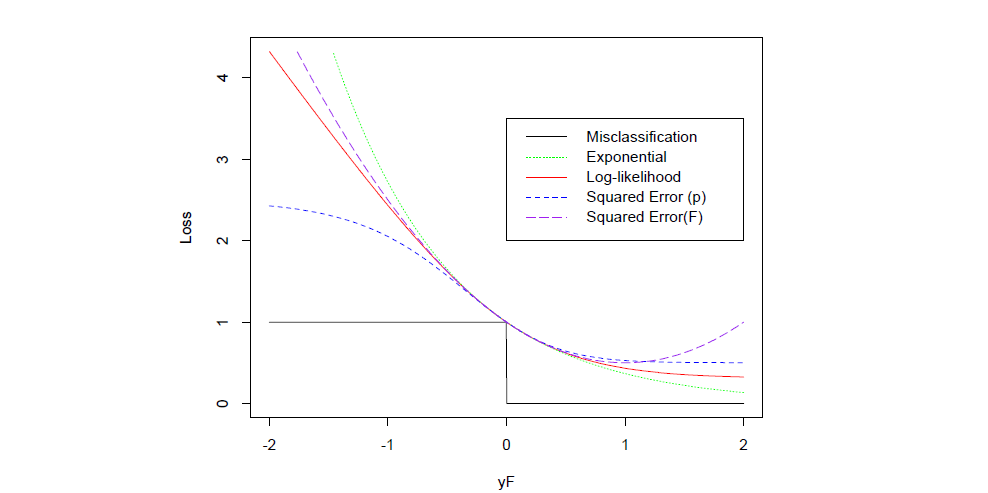
Above is a comparison between different loss function (scaled to cross(0,1)). A few take away here
- Compare with Squared Error (F), exponential loss is monotonically decreasing with \(yf(x)\), it doesn't penalize sample that are too correctly classified.
- Both exponential loss and log-likelihood penalize large negative margin \(yf(x)\) - very wrong prediction
- Exponential loss penalize negative margin even more, makes it sensitive to noise, such as mislabeled sample and outliers.
For more detailed discussion of better loss function, we will further discussion this in the following Gradient Boosting Machine, a more powerful boosting algorithm.
AdaBoost sklearn source code
Now let's go through sklearn source code and see how AdaBoost is implemented. Some modification is made to simplify the code here.
Boosting
n_estimators defines maximum of iteration. It is the maximum number of base learner in the additive model.
for iboost in range(self.n_estimators):
    # train base learner
    sample_weight, estimator_weight, estimator_error = self._boost(iboost,X, y, sample_weight, random_state)
    # store base learner error and coefficient
    self.estimator_weights_[iboost] = estimator_weight
    self.estimator_errors_[iboost] = estimator_error
    # weight normalization
    sample_weight_sum = np.sum(sample_weight)
    sample_weight /= sample_weight_sum
Base Learner
1. AdaBoostClassifier
By default AdaBoostClassifier will use DecisionTreeClassifier as base learner. For details of classification tree, you can go to my previous post - Tree - Overview of Decision Tree with sklearn source code
Sklearn support both multi-class real and discrete AdaBoost, where algorithm = 'SAMME.R' stands for real, and 'SAMME' is discrete. Here we take discrete one as example.
def _boost_discrete(self, iboost, X, y, sample_weight, random_state):
	estimator = self._make_estimator(random_state=random_state)
	estimator.fit(X, y, sample_weight=sample_weight)

	y_predict = estimator.predict(X)  # predict sample class

	incorrect = y_predict != y # get misclassified sample

	estimator_error = np.mean(np.average(incorrect, weights=sample_weight, axis=0)) # weighted misclassification rate

	estimator_weight = self.learning_rate * (
		np.log((1. - estimator_error) / estimator_error) +
		np.log(n_classes - 1.)) # coefficient of base learner in final ensemble

	sample_weight *= np.exp(estimator_weight * incorrect *
							((sample_weight > 0) |
							 (estimator_weight < 0))) # update sample weight

	return sample_weight, estimator_weight, estimator_error
2. AdaBoostRegressor
By default DecisionTreeRegressor is used as base learner for regression. Different loss functions are used: {'linear', 'square', 'exponential'}
In this post we mainly focus on classification problem. I will cover more details about regression in other ensemble algorithm.
def _boost(self, iboost, X, y, sample_weight, random_state):
	estimator = self._make_estimator(random_state=random_state)

	estimator.fit(X[bootstrap_idx], y[bootstrap_idx]) #bootstrap to create weighted sample
	y_predict = estimator.predict(X)

	error_vect = np.abs(y_predict - y)
	error_max = error_vect.max()

	if error_max != 0.:
		error_vect /= error_max # scale error by max absolute error

	if self.loss == 'square':
		error_vect **= 2
	elif self.loss == 'exponential':
		error_vect = 1. - np.exp(- error_vect)

	estimator_error = (sample_weight * error_vect).sum() # weighted average loss

    beta = estimator_error / (1. - estimator_error) #

	estimator_weight = self.learning_rate * np.log(1. / beta) # estimator coefficient

	sample_weight *= np.power(
		beta, (1. - error_vect) * self.learning_rate) # update sample with error

	return sample_weight, estimator_weight, estimator_error
Ensemble
When the model finish training, we ensemble all estimators to yield final prediction.
def decision_function(self, X):

	X = self._validate_X_predict(X)

	n_classes = self.n_classes_
	classes = self.classes_[:, np.newaxis]
	pred = None

	if self.algorithm == 'SAMME.R':
		pred = sum(_samme_proba(estimator, n_classes, X)
				   for estimator in self.estimators_) # Real doesn't coefficient
	else:
		pred = sum((estimator.predict(X) == classes).T * w
				   for estimator, w in zip(self.estimators_,
										   self.estimator_weights_)) # weighted class label

	pred /= self.estimator_weights_.sum() #normalize by weight
	if n_classes == 2:
		pred[:, 0] *= -1
		return pred.sum(axis=1)
	return pred
To be continued.
Reference
- Friedman, J., Hastie, T., and Tibshirani, R. (2000).
Special invited paper. additive logistic regression: A statistical
view of boosting - Freund, Y., Schapire, R. E., et al. (1996).
Experiments with a new boosting algorithm. - Freund, Y. and Schapire, R. E. (1997).
A decision-theoretic generalization of on-line learning and an
application to boosting. - Freund, Y. and Schapire, R. E. (1995). A desicion-theoretic generalization of online learning and an application to boosting, pages 23¨C37.
- T. Hastie, R. Tibshirani and J. Friedman. (2009). “Elements of Statistical Learning”, Springer.
- Bishop, Pattern Recognition and Machine Learning 2006
- scikit-learn tutorial http://scikit-learn.org/stable/modules/generated/sklearn.ensemble.AdaBoostClassifier.html

 浙公网安备 33010602011771号