Yolov8-源码解析-二十二-

Yolov8 源码解析（二十二）

comments: true
description: Learn how to set up and run YOLOv5 in a Docker container with step-by-step instructions. Explore other quickstart options for an easy setup.
keywords: YOLOv5, Docker, Ultralytics, setup, guide, tutorial, machine learning, deep learning, AI, GPU, NVIDIA, container

Get Started with YOLOv5 🚀 in Docker

This tutorial will guide you through the process of setting up and running YOLOv5 in a Docker container.

You can also explore other quickstart options for YOLOv5, such as our Colab Notebook , GCP Deep Learning VM, and Amazon AWS.

Prerequisites

NVIDIA Driver: Version 455.23 or higher. Download from Nvidia's website.
NVIDIA-Docker: Allows Docker to interact with your local GPU. Installation instructions are available on the NVIDIA-Docker GitHub repository.
Docker Engine - CE: Version 19.03 or higher. Download and installation instructions can be found on the Docker website.

Step 1: Pull the YOLOv5 Docker Image

The Ultralytics YOLOv5 DockerHub repository is available at https://hub.docker.com/r/ultralytics/yolov5. Docker Autobuild ensures that the ultralytics/yolov5:latest image is always in sync with the most recent repository commit. To pull the latest image, run the following command:

sudo docker pull ultralytics/yolov5:latest

Step 2: Run the Docker Container

Basic container:

Run an interactive instance of the YOLOv5 Docker image (called a "container") using the -it flag:

sudo docker run --ipc=host -it ultralytics/yolov5:latest

Container with local file access:

To run a container with access to local files (e.g., COCO training data in /datasets), use the -v flag:

sudo docker run --ipc=host -it -v "$(pwd)"/datasets:/usr/src/datasets ultralytics/yolov5:latest

Container with GPU access:

To run a container with GPU access, use the --gpus all flag:

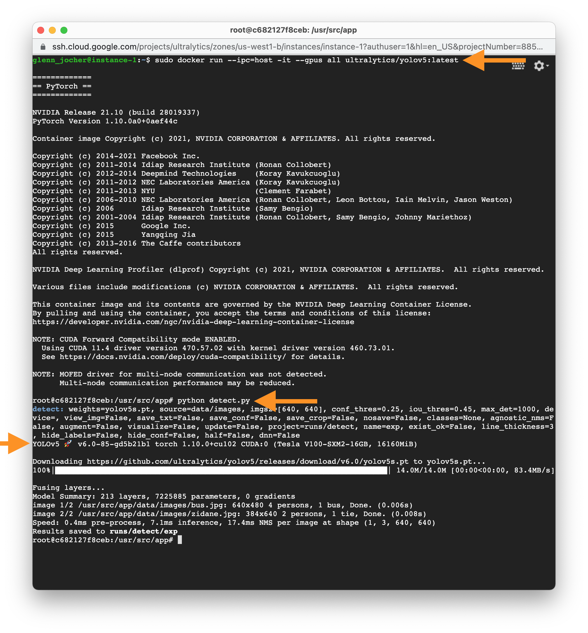
sudo docker run --ipc=host -it --gpus all ultralytics/yolov5:latest

Step 3: Use YOLOv5 🚀 within the Docker Container

Now you can train, test, detect, and export YOLOv5 models within the running Docker container:

# Train a model on your data
python train.py

# Validate the trained model for Precision, Recall, and mAP
python val.py --weights yolov5s.pt

# Run inference using the trained model on your images or videos
python detect.py --weights yolov5s.pt --source path/to/images

# Export the trained model to other formats for deployment
python export.py --weights yolov5s.pt --include onnx coreml tflite

comments: true
description: Master YOLOv5 deployment on Google Cloud Platform Deep Learning VM. Perfect for AI beginners and experts to achieve high-performance object detection.
keywords: YOLOv5, Google Cloud Platform, GCP, Deep Learning VM, object detection, AI, machine learning, tutorial

Mastering YOLOv5 🚀 Deployment on Google Cloud Platform (GCP) Deep Learning Virtual Machine (VM) ⭐

Embarking on the journey of artificial intelligence and machine learning can be exhilarating, especially when you leverage the power and flexibility of a cloud platform. Google Cloud Platform (GCP) offers robust tools tailored for machine learning enthusiasts and professionals alike. One such tool is the Deep Learning VM that is preconfigured for data science and ML tasks. In this tutorial, we will navigate through the process of setting up YOLOv5 on a GCP Deep Learning VM. Whether you're taking your first steps in ML or you're a seasoned practitioner, this guide is designed to provide you with a clear pathway to implementing object detection models powered by YOLOv5.

🆓 Plus, if you're a fresh GCP user, you're in luck with a $300 free credit offer to kickstart your projects.

In addition to GCP, explore other accessible quickstart options for YOLOv5, like our Colab Notebook for a browser-based experience, or the scalability of Amazon AWS. Furthermore, container aficionados can utilize our official Docker image at Docker Hub for an encapsulated environment.

Step 1: Create and Configure Your Deep Learning VM

Let's begin by creating a virtual machine that's tuned for deep learning:

Head over to the GCP marketplace and select the Deep Learning VM.
Opt for a n1-standard-8 instance; it offers a balance of 8 vCPUs and 30 GB of memory, ideally suited for our needs.
Next, select a GPU. This depends on your workload; even a basic one like the Tesla T4 will markedly accelerate your model training.
Tick the box for 'Install NVIDIA GPU driver automatically on first startup?' for hassle-free setup.
Allocate a 300 GB SSD Persistent Disk to ensure you don't bottleneck on I/O operations.
Hit 'Deploy' and let GCP do its magic in provisioning your custom Deep Learning VM.

This VM comes loaded with a treasure trove of preinstalled tools and frameworks, including the Anaconda Python distribution, which conveniently bundles all the necessary dependencies for YOLOv5.

Step 2: Ready the VM for YOLOv5

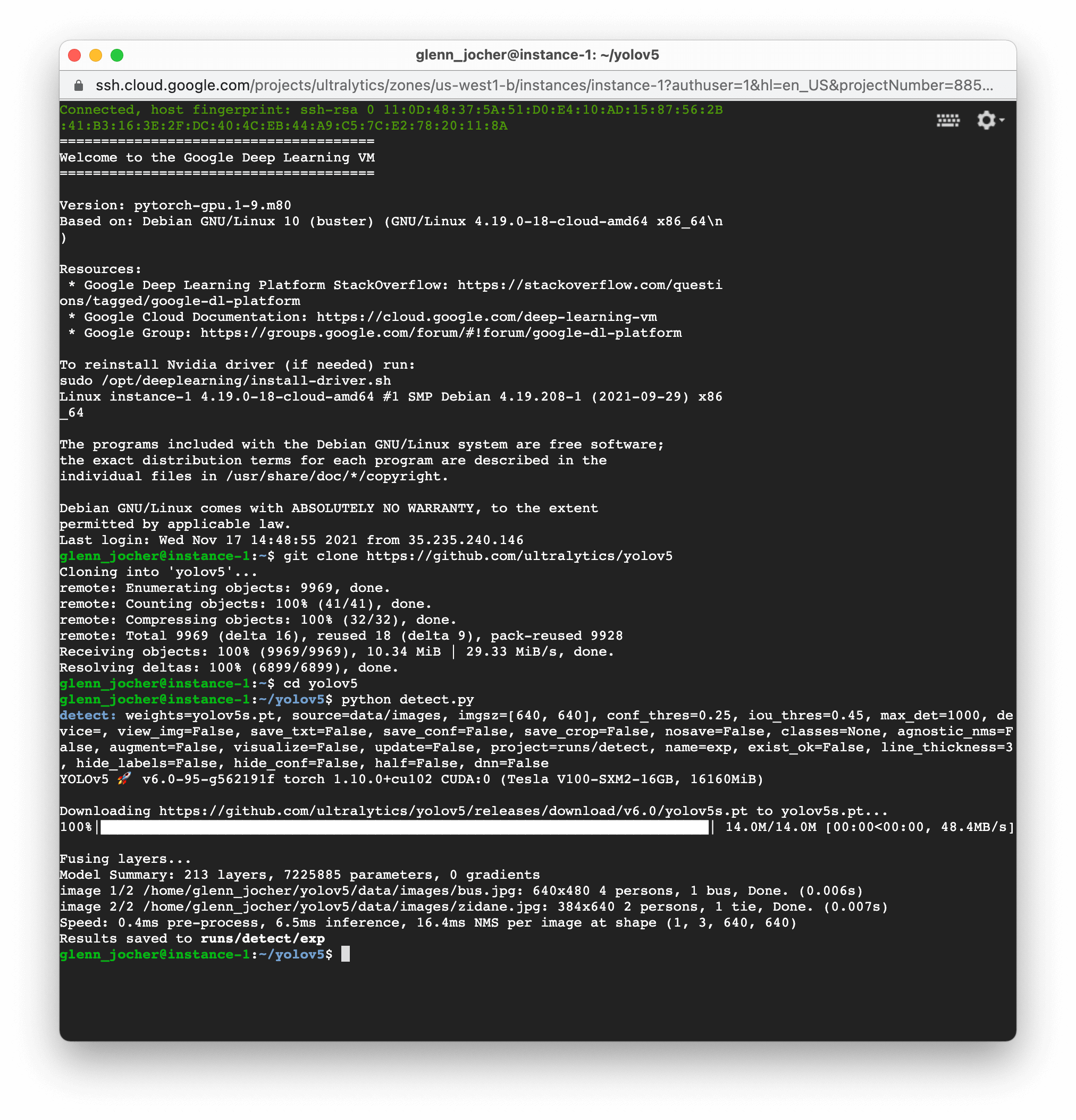
Following the environment setup, let's get YOLOv5 up and running:

# Clone the YOLOv5 repository
git clone https://github.com/ultralytics/yolov5

# Change the directory to the cloned repository
cd yolov5

# Install the necessary Python packages from requirements.txt
pip install -r requirements.txt

This setup process ensures you're working with a Python environment version 3.8.0 or newer and PyTorch 1.8 or above. Our scripts smoothly download models and datasets rending from the latest YOLOv5 release, making it hassle-free to start model training.

Step 3: Train and Deploy Your YOLOv5 Models 🌐

With the setup complete, you're ready to delve into training and inference with YOLOv5 on your GCP VM:

# Train a model on your data
python train.py

# Validate the trained model for Precision, Recall, and mAP
python val.py --weights yolov5s.pt

# Run inference using the trained model on your images or videos
python detect.py --weights yolov5s.pt --source path/to/images

# Export the trained model to other formats for deployment
python export.py --weights yolov5s.pt --include onnx coreml tflite

With just a few commands, YOLOv5 allows you to train custom object detection models tailored to your specific needs or utilize pre-trained weights for quick results on a variety of tasks.

Allocate Swap Space (optional)

For those dealing with hefty datasets, consider amplifying your GCP instance with an additional 64GB of swap memory:

sudo fallocate -l 64G /swapfile
sudo chmod 600 /swapfile
sudo mkswap /swapfile
sudo swapon /swapfile
free -h  # confirm the memory increment

Concluding Thoughts

Congratulations! You are now empowered to harness the capabilities of YOLOv5 with the computational prowess of Google Cloud Platform. This combination provides scalability, efficiency, and versatility for your object detection tasks. Whether for personal projects, academic research, or industrial applications, you have taken a pivotal step into the world of AI and machine learning on the cloud.

Do remember to document your journey, share insights with the Ultralytics community, and leverage the collaborative arenas such as GitHub discussions to grow further. Now, go forth and innovate with YOLOv5 and GCP! 🌟

Want to keep improving your ML skills and knowledge? Dive into our documentation and tutorials for more resources. Let your AI adventure continue!

comments: true
description: Explore comprehensive YOLOv5 documentation with step-by-step tutorials on training, deployment, and model optimization. Empower your vision projects today!.
keywords: YOLOv5, Ultralytics, object detection, computer vision, deep learning, AI, tutorials, PyTorch, model optimization, machine learning, neural networks

Comprehensive Guide to Ultralytics YOLOv5

Welcome to the Ultralytics' YOLOv5🚀 Documentation! YOLOv5, the fifth iteration of the revolutionary "You Only Look Once" object detection model, is designed to deliver high-speed, high-accuracy results in real-time.

Built on PyTorch, this powerful deep learning framework has garnered immense popularity for its versatility, ease of use, and high performance. Our documentation guides you through the installation process, explains the architectural nuances of the model, showcases various use-cases, and provides a series of detailed tutorials. These resources will help you harness the full potential of YOLOv5 for your computer vision projects. Let's get started!

Explore and Learn

Here's a compilation of comprehensive tutorials that will guide you through different aspects of YOLOv5.

Train Custom Data 🚀 RECOMMENDED: Learn how to train the YOLOv5 model on your custom dataset.
Tips for Best Training Results ☘️: Uncover practical tips to optimize your model training process.
Multi-GPU Training: Understand how to leverage multiple GPUs to expedite your training.
PyTorch Hub 🌟 NEW: Learn to load pre-trained models via PyTorch Hub.
TFLite, ONNX, CoreML, TensorRT Export 🚀: Understand how to export your model to different formats.
Test-Time Augmentation (TTA): Explore how to use TTA to improve your model's prediction accuracy.
Model Ensembling: Learn the strategy of combining multiple models for improved performance.
Model Pruning/Sparsity: Understand pruning and sparsity concepts, and how to create a more efficient model.
Hyperparameter Evolution: Discover the process of automated hyperparameter tuning for better model performance.
Transfer Learning with Frozen Layers: Learn how to implement transfer learning by freezing layers in YOLOv5.
Architecture Summary 🌟 Delve into the structural details of the YOLOv5 model.
Roboflow for Datasets: Understand how to utilize Roboflow for dataset management, labeling, and active learning.
ClearML Logging 🌟 Learn how to integrate ClearML for efficient logging during your model training.
YOLOv5 with Neural Magic Discover how to use Neural Magic's Deepsparse to prune and quantize your YOLOv5 model.
Comet Logging 🌟 NEW: Explore how to utilize Comet for improved model training logging.

Supported Environments

Ultralytics provides a range of ready-to-use environments, each pre-installed with essential dependencies such as CUDA, CUDNN, Python, and PyTorch, to kickstart your projects.

Free GPU Notebooks:
Google Cloud: GCP Quickstart Guide
Amazon: AWS Quickstart Guide
Azure: AzureML Quickstart Guide
Docker: Docker Quickstart Guide

Project Status

This badge indicates that all YOLOv5 GitHub Actions Continuous Integration (CI) tests are successfully passing. These CI tests rigorously check the functionality and performance of YOLOv5 across various key aspects: training, validation, inference, export, and benchmarks. They ensure consistent and reliable operation on macOS, Windows, and Ubuntu, with tests conducted every 24 hours and upon each new commit.

Connect and Contribute

Your journey with YOLOv5 doesn't have to be a solitary one. Join our vibrant community on GitHub, connect with professionals on LinkedIn, share your results on Twitter, and find educational resources on YouTube. Follow us on TikTok and BiliBili for more engaging content.

Interested in contributing? We welcome contributions of all forms; from code improvements and bug reports to documentation updates. Check out our contributing guidelines for more information.

We're excited to see the innovative ways you'll use YOLOv5. Dive in, experiment, and revolutionize your computer vision projects! 🚀

FAQ

What are the key features of Ultralytics YOLOv5?

Ultralytics YOLOv5 is renowned for its high-speed and high-accuracy object detection capabilities. Built on PyTorch, it is versatile and user-friendly, making it suitable for various computer vision projects. Key features include real-time inference, support for multiple training tricks like Test-Time Augmentation (TTA) and Model Ensembling, and compatibility with export formats such as TFLite, ONNX, CoreML, and TensorRT. To delve deeper into how Ultralytics YOLOv5 can elevate your project, explore our TFLite, ONNX, CoreML, TensorRT Export guide.

How can I train a custom YOLOv5 model on my dataset?

Training a custom YOLOv5 model on your dataset involves a few key steps. First, prepare your dataset in the required format, annotated with labels. Then, configure the YOLOv5 training parameters and start the training process using the train.py script. For an in-depth tutorial on this process, consult our Train Custom Data guide. It provides step-by-step instructions to ensure optimal results for your specific use case.

Why should I use Ultralytics YOLOv5 over other object detection models like RCNN?

Ultralytics YOLOv5 is preferred over models like RCNN due to its superior speed and accuracy in real-time object detection. YOLOv5 processes the entire image in one go, making it significantly faster compared to the region-based approach of RCNN, which involves multiple passes. Additionally, YOLOv5's seamless integration with various export formats and extensive documentation make it an excellent choice for both beginners and professionals. Learn more about the architectural advantages in our Architecture Summary.

How can I optimize YOLOv5 model performance during training?

Optimizing YOLOv5 model performance involves tuning various hyperparameters and incorporating techniques like data augmentation and transfer learning. Ultralytics provides comprehensive resources on hyperparameter evolution and pruning/sparsity to improve model efficiency. You can discover practical tips in our Tips for Best Training Results guide, which offers actionable insights for achieving optimal performance during training.

What environments are supported for running YOLOv5 applications?

Ultralytics YOLOv5 supports a variety of environments, including free GPU notebooks on Gradient, Google Colab, Kaggle, as well as major cloud platforms like Google Cloud, Amazon AWS, and Azure. Docker images are also available for convenient setup. For a detailed guide on setting up these environments, check our Supported Environments section, which includes step-by-step instructions for each platform.

comments: true
description: Kickstart your real-time object detection journey with YOLOv5! This guide covers installation, inference, and training to help you master YOLOv5 quickly.
keywords: YOLOv5, Quickstart, real-time object detection, AI, ML, PyTorch, inference, training, Ultralytics, machine learning, deep learning

YOLOv5 Quickstart 🚀

Embark on your journey into the dynamic realm of real-time object detection with YOLOv5! This guide is crafted to serve as a comprehensive starting point for AI enthusiasts and professionals aiming to master YOLOv5. From initial setup to advanced training techniques, we've got you covered. By the end of this guide, you'll have the knowledge to implement YOLOv5 into your projects confidently. Let's ignite the engines and soar into YOLOv5!

Install

Prepare for launch by cloning the repository and establishing the environment. This ensures that all the necessary requirements are installed. Check that you have Python>=3.8.0 and PyTorch>=1.8 ready for takeoff.

git clone https://github.com/ultralytics/yolov5  # clone repository
cd yolov5
pip install -r requirements.txt  # install dependencies

Inference with PyTorch Hub

Experience the simplicity of YOLOv5 PyTorch Hub inference, where models are seamlessly downloaded from the latest YOLOv5 release.

import torch

# Model loading
model = torch.hub.load("ultralytics/yolov5", "yolov5s")  # Can be 'yolov5n' - 'yolov5x6', or 'custom'

# Inference on images
img = "https://ultralytics.com/images/zidane.jpg"  # Can be a file, Path, PIL, OpenCV, numpy, or list of images

# Run inference
results = model(img)

# Display results
results.print()  # Other options: .show(), .save(), .crop(), .pandas(), etc.

Inference with detect.py

Harness detect.py for versatile inference on various sources. It automatically fetches models from the latest YOLOv5 release and saves results with ease.

python detect.py --weights yolov5s.pt --source 0                               # webcam
                                               img.jpg                         # image
                                               vid.mp4                         # video
                                               screen                          # screenshot
                                               path/                           # directory
                                               list.txt                        # list of images
                                               list.streams                    # list of streams
                                               'path/*.jpg'                    # glob
                                               'https://youtu.be/LNwODJXcvt4'  # YouTube
                                               'rtsp://example.com/media.mp4'  # RTSP, RTMP, HTTP stream

Training

Replicate the YOLOv5 COCO benchmarks with the instructions below. The necessary models and datasets are pulled directly from the latest YOLOv5 release. Training YOLOv5n/s/m/l/x on a V100 GPU should typically take 1/2/4/6/8 days respectively (note that Multi-GPU setups work faster). Maximize performance by using the highest possible --batch-size or use --batch-size -1 for the YOLOv5 AutoBatch feature. The following batch sizes are ideal for V100-16GB GPUs.

python train.py --data coco.yaml --epochs 300 --weights '' --cfg yolov5n.yaml  --batch-size 128
                                                                 yolov5s                    64
                                                                 yolov5m                    40
                                                                 yolov5l                    24
                                                                 yolov5x                    16

To conclude, YOLOv5 is not only a state-of-the-art tool for object detection but also a testament to the power of machine learning in transforming the way we interact with the world through visual understanding. As you progress through this guide and begin applying YOLOv5 to your projects, remember that you are at the forefront of a technological revolution, capable of achieving remarkable feats. Should you need further insights or support from fellow visionaries, you're invited to our GitHub repository home to a thriving community of developers and researchers. Keep exploring, keep innovating, and enjoy the marvels of YOLOv5. Happy detecting! 🌠🔍

comments: true
description: Dive deep into the powerful YOLOv5 architecture by Ultralytics, exploring its model structure, data augmentation techniques, training strategies, and loss computations.
keywords: YOLOv5 architecture, object detection, Ultralytics, YOLO, model structure, data augmentation, training strategies, loss computations, deep learning, machine learning

Ultralytics YOLOv5 Architecture

YOLOv5 (v6.0/6.1) is a powerful object detection algorithm developed by Ultralytics. This article dives deep into the YOLOv5 architecture, data augmentation strategies, training methodologies, and loss computation techniques. This comprehensive understanding will help improve your practical application of object detection in various fields, including surveillance, autonomous vehicles, and image recognition.

1. Model Structure

YOLOv5's architecture consists of three main parts:

Backbone: This is the main body of the network. For YOLOv5, the backbone is designed using the New CSP-Darknet53 structure, a modification of the Darknet architecture used in previous versions.
Neck: This part connects the backbone and the head. In YOLOv5, SPPF and New CSP-PAN structures are utilized.
Head: This part is responsible for generating the final output. YOLOv5 uses the YOLOv3 Head for this purpose.

The structure of the model is depicted in the image below. The model structure details can be found in yolov5l.yaml.

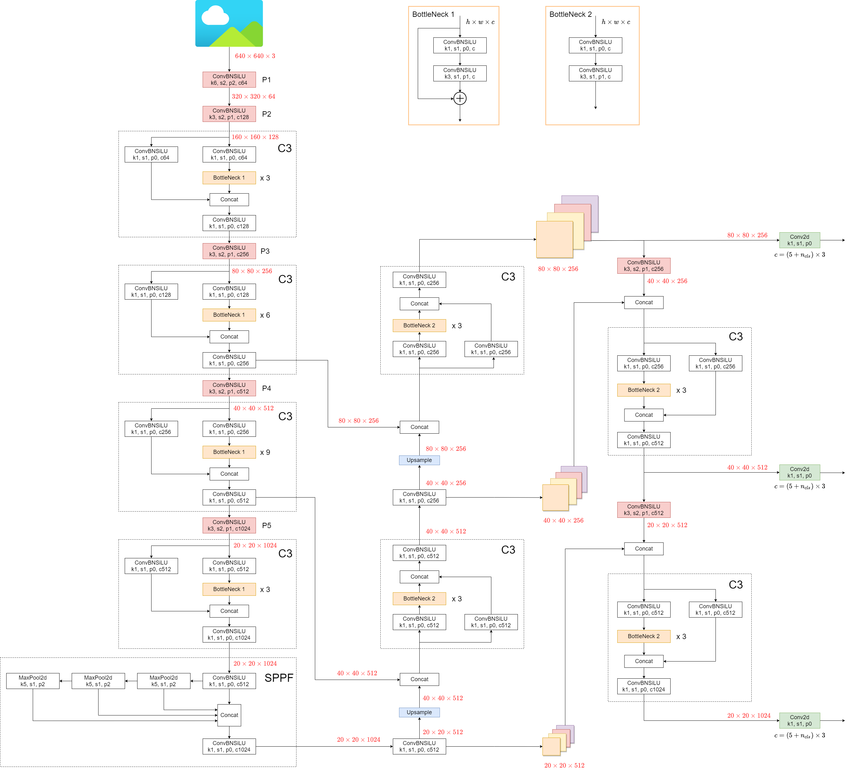
YOLOv5 introduces some minor changes compared to its predecessors:

The Focus structure, found in earlier versions, is replaced with a 6x6 Conv2d structure. This change boosts efficiency #4825.
The SPP structure is replaced with SPPF. This alteration more than doubles the speed of processing.

To test the speed of SPP and SPPF, the following code can be used:

SPP vs SPPF speed profiling example (click to open)

import time

import torch
import torch.nn as nn


class SPP(nn.Module):
    def __init__(self):
        """Initializes an SPP module with three different sizes of max pooling layers."""
        super().__init__()
        self.maxpool1 = nn.MaxPool2d(5, 1, padding=2)
        self.maxpool2 = nn.MaxPool2d(9, 1, padding=4)
        self.maxpool3 = nn.MaxPool2d(13, 1, padding=6)

    def forward(self, x):
        """Applies three max pooling layers on input `x` and concatenates results along channel dimension."""
        o1 = self.maxpool1(x)
        o2 = self.maxpool2(x)
        o3 = self.maxpool3(x)
        return torch.cat([x, o1, o2, o3], dim=1)


class SPPF(nn.Module):
    def __init__(self):
        """Initializes an SPPF module with a specific configuration of MaxPool2d layer."""
        super().__init__()
        self.maxpool = nn.MaxPool2d(5, 1, padding=2)

    def forward(self, x):
        """Applies sequential max pooling and concatenates results with input tensor."""
        o1 = self.maxpool(x)
        o2 = self.maxpool(o1)
        o3 = self.maxpool(o2)
        return torch.cat([x, o1, o2, o3], dim=1)


def main():
    """Compares outputs and performance of SPP and SPPF on a random tensor (8, 32, 16, 16)."""
    input_tensor = torch.rand(8, 32, 16, 16)
    spp = SPP()
    sppf = SPPF()
    output1 = spp(input_tensor)
    output2 = sppf(input_tensor)

    print(torch.equal(output1, output2))

    t_start = time.time()
    for _ in range(100):
        spp(input_tensor)
    print(f"SPP time: {time.time() - t_start}")

    t_start = time.time()
    for _ in range(100):
        sppf(input_tensor)
    print(f"SPPF time: {time.time() - t_start}")


if __name__ == "__main__":
    main()

result:

True
SPP time: 0.5373051166534424
SPPF time: 0.20780706405639648

2. Data Augmentation Techniques

YOLOv5 employs various data augmentation techniques to improve the model's ability to generalize and reduce overfitting. These techniques include:

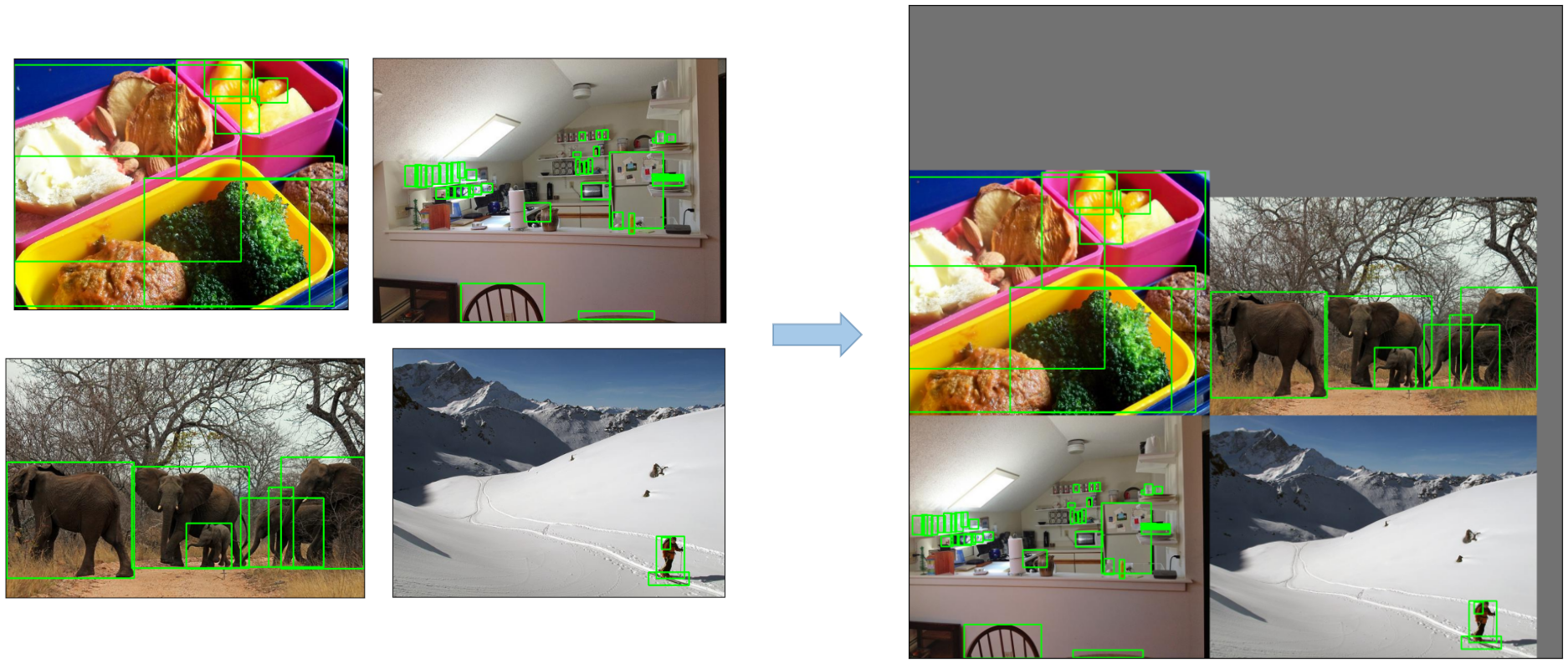
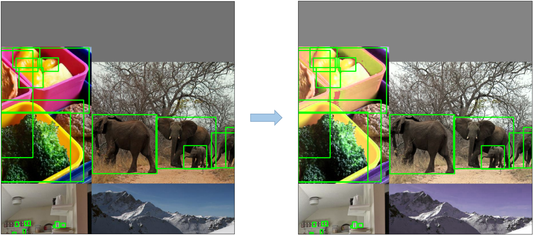
Mosaic Augmentation: An image processing technique that combines four training images into one in ways that encourage object detection models to better handle various object scales and translations.
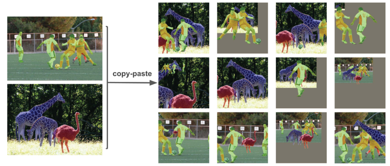
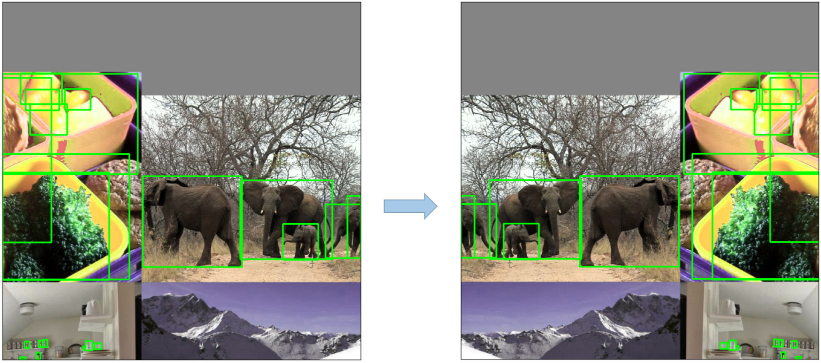
Copy-Paste Augmentation: An innovative data augmentation method that copies random patches from an image and pastes them onto another randomly chosen image, effectively generating a new training sample.
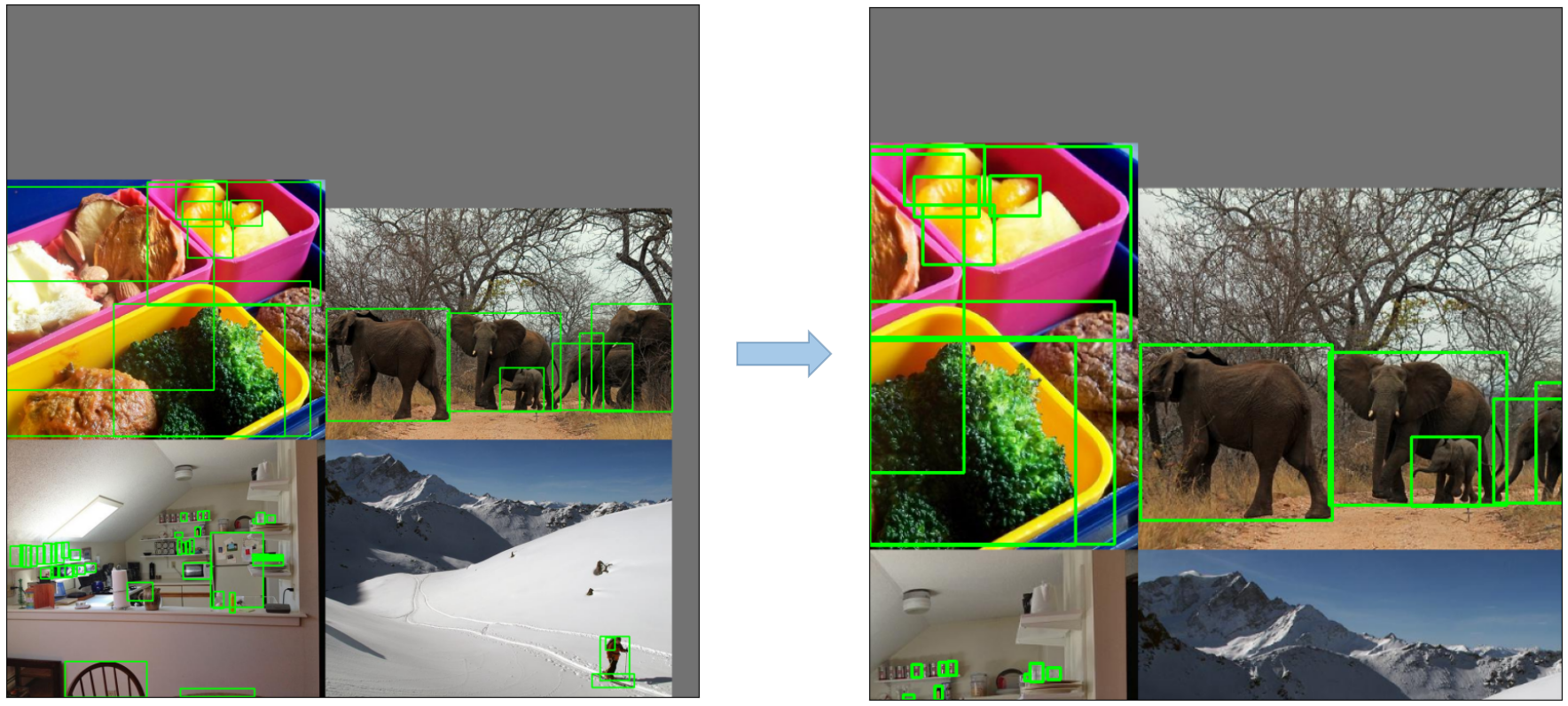
Random Affine Transformations: This includes random rotation, scaling, translation, and shearing of the images.
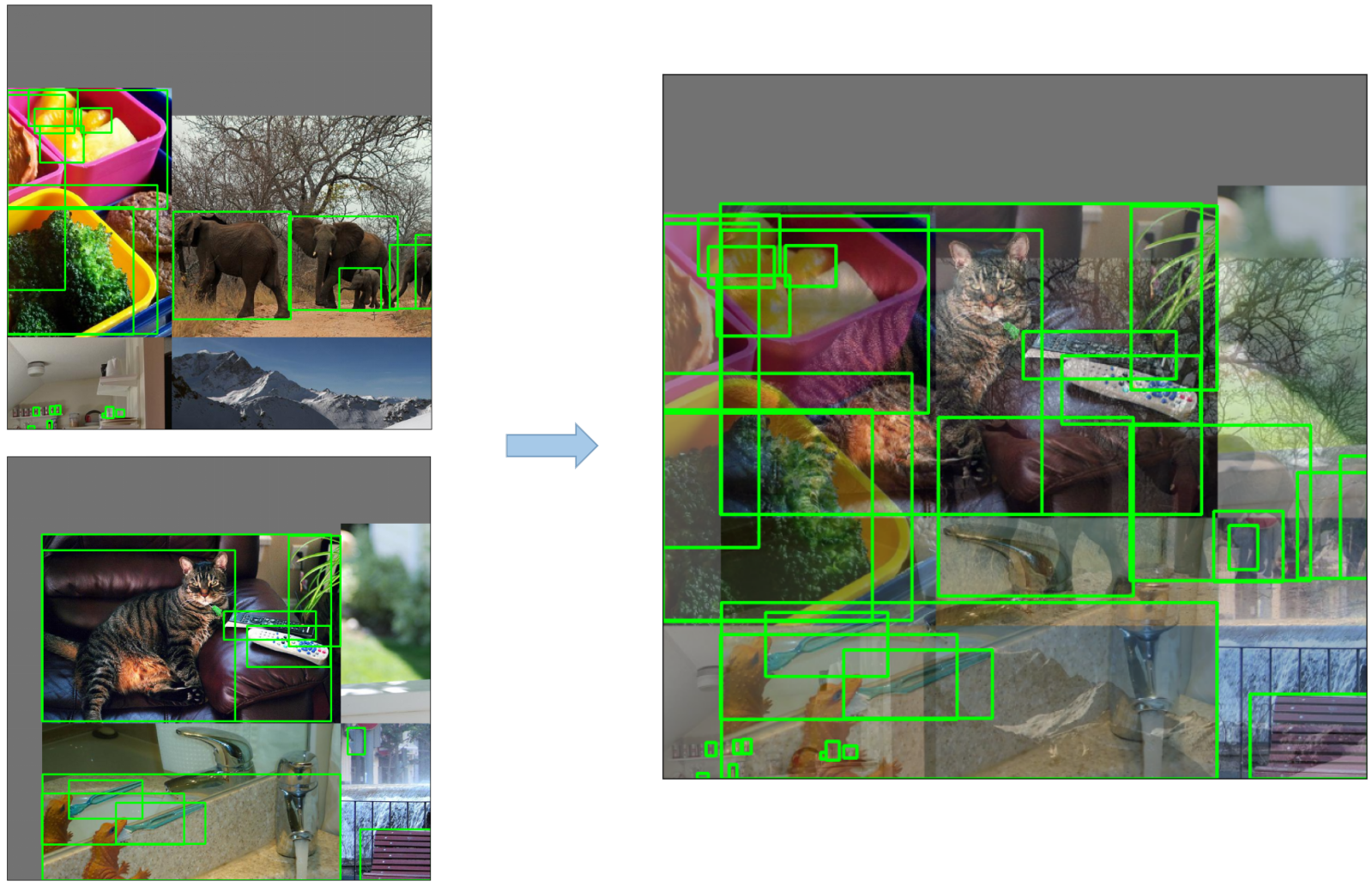
MixUp Augmentation: A method that creates composite images by taking a linear combination of two images and their associated labels.
Albumentations: A powerful library for image augmenting that supports a wide variety of augmentation techniques.
HSV Augmentation: Random changes to the Hue, Saturation, and Value of the images.
Random Horizontal Flip: An augmentation method that randomly flips images horizontally.

3. Training Strategies

YOLOv5 applies several sophisticated training strategies to enhance the model's performance. They include:

Multiscale Training: The input images are randomly rescaled within a range of 0.5 to 1.5 times their original size during the training process.
AutoAnchor: This strategy optimizes the prior anchor boxes to match the statistical characteristics of the ground truth boxes in your custom data.
Warmup and Cosine LR Scheduler: A method to adjust the learning rate to enhance model performance.
Exponential Moving Average (EMA): A strategy that uses the average of parameters over past steps to stabilize the training process and reduce generalization error.
Mixed Precision Training: A method to perform operations in half-precision format, reducing memory usage and enhancing computational speed.
Hyperparameter Evolution: A strategy to automatically tune hyperparameters to achieve optimal performance.

4. Additional Features

4.1 Compute Losses

The loss in YOLOv5 is computed as a combination of three individual loss components:

Classes Loss (BCE Loss): Binary Cross-Entropy loss, measures the error for the classification task.
Objectness Loss (BCE Loss): Another Binary Cross-Entropy loss, calculates the error in detecting whether an object is present in a particular grid cell or not.
Location Loss (CIoU Loss): Complete IoU loss, measures the error in localizing the object within the grid cell.

The overall loss function is depicted by:

4.2 Balance Losses

The objectness losses of the three prediction layers (P3, P4, P5) are weighted differently. The balance weights are [4.0, 1.0, 0.4] respectively. This approach ensures that the predictions at different scales contribute appropriately to the total loss.

4.3 Eliminate Grid Sensitivity

The YOLOv5 architecture makes some important changes to the box prediction strategy compared to earlier versions of YOLO. In YOLOv2 and YOLOv3, the box coordinates were directly predicted using the activation of the last layer.

However, in YOLOv5, the formula for predicting the box coordinates has been updated to reduce grid sensitivity and prevent the model from predicting unbounded box dimensions.

The revised formulas for calculating the predicted bounding box are as follows:

Compare the center point offset before and after scaling. The center point offset range is adjusted from (0, 1) to (-0.5, 1.5). Therefore, offset can easily get 0 or 1.

Compare the height and width scaling ratio(relative to anchor) before and after adjustment. The original yolo/darknet box equations have a serious flaw. Width and Height are completely unbounded as they are simply out=exp(in), which is dangerous, as it can lead to runaway gradients, instabilities, NaN losses and ultimately a complete loss of training. refer this issue

4.4 Build Targets

The build target process in YOLOv5 is critical for training efficiency and model accuracy. It involves assigning ground truth boxes to the appropriate grid cells in the output map and matching them with the appropriate anchor boxes.

This process follows these steps:

Calculate the ratio of the ground truth box dimensions and the dimensions of each anchor template.

If the calculated ratio is within the threshold, match the ground truth box with the corresponding anchor.

Assign the matched anchor to the appropriate cells, keeping in mind that due to the revised center point offset, a ground truth box can be assigned to more than one anchor. Because the center point offset range is adjusted from (0, 1) to (-0.5, 1.5). GT Box can be assigned to more anchors.

This way, the build targets process ensures that each ground truth object is properly assigned and matched during the training process, allowing YOLOv5 to learn the task of object detection more effectively.

Conclusion

In conclusion, YOLOv5 represents a significant step forward in the development of real-time object detection models. By incorporating various new features, enhancements, and training strategies, it surpasses previous versions of the YOLO family in performance and efficiency.

The primary enhancements in YOLOv5 include the use of a dynamic architecture, an extensive range of data augmentation techniques, innovative training strategies, as well as important adjustments in computing losses and the process of building targets. All these innovations significantly improve the accuracy and efficiency of object detection while retaining a high degree of speed, which is the trademark of YOLO models.

comments: true
description: Learn how to use ClearML for tracking YOLOv5 experiments, data versioning, hyperparameter optimization, and remote execution with ease.
keywords: ClearML, YOLOv5, machine learning, experiment tracking, data versioning, hyperparameter optimization, remote execution, ML pipeline

ClearML Integration

About ClearML

ClearML is an open-source toolbox designed to save you time ⏱️.

🔨 Track every YOLOv5 training run in the experiment manager

🔧 Version and easily access your custom training data with the integrated ClearML Data Versioning Tool

🔦 Remotely train and monitor your YOLOv5 training runs using ClearML Agent

🔬 Get the very best mAP using ClearML Hyperparameter Optimization

🔭 Turn your newly trained YOLOv5 model into an API with just a few commands using ClearML Serving

And so much more. It's up to you how many of these tools you want to use, you can stick to the experiment manager, or chain them all together into an impressive pipeline!

🦾 Setting Things Up

To keep track of your experiments and/or data, ClearML needs to communicate to a server. You have 2 options to get one:

Either sign up for free to the ClearML Hosted Service or you can set up your own server, see here. Even the server is open-source, so even if you're dealing with sensitive data, you should be good to go!

Install the clearml python package:
```
pip install clearml
```
Connect the ClearML SDK to the server by creating credentials (go right top to Settings -> Workspace -> Create new credentials), then execute the command below and follow the instructions:
```
clearml-init
```

That's it! You're done 😎

🚀 Training YOLOv5 With ClearML

To enable ClearML experiment tracking, simply install the ClearML pip package.

pip install clearml>=1.2.0

This will enable integration with the YOLOv5 training script. Every training run from now on, will be captured and stored by the ClearML experiment manager.

If you want to change the project_name or task_name, use the --project and --name arguments of the train.py script, by default the project will be called YOLOv5 and the task Training. PLEASE NOTE: ClearML uses / as a delimiter for subprojects, so be careful when using / in your project name!

python train.py --img 640 --batch 16 --epochs 3 --data coco8.yaml --weights yolov5s.pt --cache

or with custom project and task name:

python train.py --project my_project --name my_training --img 640 --batch 16 --epochs 3 --data coco8.yaml --weights yolov5s.pt --cache

This will capture:

Source code + uncommitted changes
Installed packages
(Hyper)parameters
Model files (use --save-period n to save a checkpoint every n epochs)
Console output
Scalars (mAP_0.5, mAP_0.5:0.95, precision, recall, losses, learning rates, ...)
General info such as machine details, runtime, creation date etc.
All produced plots such as label correlogram and confusion matrix
Images with bounding boxes per epoch
Mosaic per epoch
Validation images per epoch

That's a lot right? 🤯 Now, we can visualize all of this information in the ClearML UI to get an overview of our training progress. Add custom columns to the table view (such as e.g. mAP_0.5) so you can easily sort on the best performing model. Or select multiple experiments and directly compare them!

There even more we can do with all of this information, like hyperparameter optimization and remote execution, so keep reading if you want to see how that works!

🔗 Dataset Version Management

Versioning your data separately from your code is generally a good idea and makes it easy to acquire the latest version too. This repository supports supplying a dataset version ID, and it will make sure to get the data if it's not there yet. Next to that, this workflow also saves the used dataset ID as part of the task parameters, so you will always know for sure which data was used in which experiment!

Prepare Your Dataset

The YOLOv5 repository supports a number of different datasets by using YAML files containing their information. By default datasets are downloaded to the ../datasets folder in relation to the repository root folder. So if you downloaded the coco128 dataset using the link in the YAML or with the scripts provided by yolov5, you get this folder structure:

..
|_ yolov5
|_ datasets
    |_ coco128
        |_ images
        |_ labels
        |_ LICENSE
        |_ README.txt

But this can be any dataset you wish. Feel free to use your own, as long as you keep to this folder structure.

Next, ⚠️copy the corresponding YAML file to the root of the dataset folder⚠️. This YAML files contains the information ClearML will need to properly use the dataset. You can make this yourself too, of course, just follow the structure of the example YAMLs.

Basically we need the following keys: path, train, test, val, nc, names.

..
|_ yolov5
|_ datasets
    |_ coco128
        |_ images
        |_ labels
        |_ coco128.yaml  # <---- HERE!
        |_ LICENSE
        |_ README.txt

Upload Your Dataset

To get this dataset into ClearML as a versioned dataset, go to the dataset root folder and run the following command:

cd coco128
clearml-data sync --project YOLOv5 --name coco128 --folder .

The command clearml-data sync is actually a shorthand command. You could also run these commands one after the other:

# Optionally add --parent <parent_dataset_id> if you want to base
# this version on another dataset version, so no duplicate files are uploaded!
clearml-data create --name coco128 --project YOLOv5
clearml-data add --files .
clearml-data close

Run Training Using A ClearML Dataset

Now that you have a ClearML dataset, you can very simply use it to train custom YOLOv5 🚀 models!

python train.py --img 640 --batch 16 --epochs 3 --data clearml://<your_dataset_id> --weights yolov5s.pt --cache

👀 Hyperparameter Optimization

Now that we have our experiments and data versioned, it's time to take a look at what we can build on top!

Using the code information, installed packages and environment details, the experiment itself is now completely reproducible. In fact, ClearML allows you to clone an experiment and even change its parameters. We can then just rerun it with these new parameters automatically, this is basically what HPO does!

To run hyperparameter optimization locally, we've included a pre-made script for you. Just make sure a training task has been run at least once, so it is in the ClearML experiment manager, we will essentially clone it and change its hyperparameters.

You'll need to fill in the ID of this template task in the script found at utils/loggers/clearml/hpo.py and then just run it 😃 You can change task.execute_locally() to task.execute() to put it in a ClearML queue and have a remote agent work on it instead.

# To use optuna, install it first, otherwise you can change the optimizer to just be RandomSearch
pip install optuna
python utils/loggers/clearml/hpo.py

🤯 Remote Execution (advanced)

Running HPO locally is really handy, but what if we want to run our experiments on a remote machine instead? Maybe you have access to a very powerful GPU machine on-site, or you have some budget to use cloud GPUs. This is where the ClearML Agent comes into play. Check out what the agent can do here:

In short: every experiment tracked by the experiment manager contains enough information to reproduce it on a different machine (installed packages, uncommitted changes etc.). So a ClearML agent does just that: it listens to a queue for incoming tasks and when it finds one, it recreates the environment and runs it while still reporting scalars, plots etc. to the experiment manager.

You can turn any machine (a cloud VM, a local GPU machine, your own laptop ... ) into a ClearML agent by simply running:

clearml-agent daemon --queue <queues_to_listen_to> [--docker]

Cloning, Editing And Enqueuing

With our agent running, we can give it some work. Remember from the HPO section that we can clone a task and edit the hyperparameters? We can do that from the interface too!

🪄 Clone the experiment by right-clicking it

🎯 Edit the hyperparameters to what you wish them to be

⏳ Enqueue the task to any of the queues by right-clicking it

Executing A Task Remotely

Now you can clone a task like we explained above, or simply mark your current script by adding task.execute_remotely() and on execution it will be put into a queue, for the agent to start working on!

To run the YOLOv5 training script remotely, all you have to do is add this line to the training.py script after the clearml logger has been instantiated:

# ...
# Loggers
data_dict = None
if RANK in {-1, 0}:
    loggers = Loggers(save_dir, weights, opt, hyp, LOGGER)  # loggers instance
    if loggers.clearml:
        loggers.clearml.task.execute_remotely(queue="my_queue")  # <------ ADD THIS LINE
        # Data_dict is either None is user did not choose for ClearML dataset or is filled in by ClearML
        data_dict = loggers.clearml.data_dict
# ...

When running the training script after this change, python will run the script up until that line, after which it will package the code and send it to the queue instead!

Autoscaling workers

ClearML comes with autoscalers too! This tool will automatically spin up new remote machines in the cloud of your choice (AWS, GCP, Azure) and turn them into ClearML agents for you whenever there are experiments detected in the queue. Once the tasks are processed, the autoscaler will automatically shut down the remote machines, and you stop paying!

Check out the autoscalers getting started video below.

comments: true
description: Learn to track, visualize and optimize YOLOv5 model metrics with Comet for seamless machine learning workflows.
keywords: YOLOv5, Comet, machine learning, model tracking, hyperparameters, visualization, deep learning, logging, metrics

YOLOv5 with Comet

This guide will cover how to use YOLOv5 with Comet

About Comet

Comet builds tools that help data scientists, engineers, and team leaders accelerate and optimize machine learning and deep learning models.

Track and visualize model metrics in real time, save your hyperparameters, datasets, and model checkpoints, and visualize your model predictions with Comet Custom Panels! Comet makes sure you never lose track of your work and makes it easy to share results and collaborate across teams of all sizes!

Getting Started

Install Comet

pip install comet_ml

Configure Comet Credentials

There are two ways to configure Comet with YOLOv5.

You can either set your credentials through environment variables

Environment Variables

export COMET_API_KEY=<Your Comet API Key>
export COMET_PROJECT_NAME=<Your Comet Project Name> # This will default to 'yolov5'

Or create a .comet.config file in your working directory and set your credentials there.

Comet Configuration File

[comet]
api_key=<Your Comet API Key>
project_name=<Your Comet Project Name> # This will default to 'yolov5'

Run the Training Script

# Train YOLOv5s on COCO128 for 5 epochs
python train.py --img 640 --batch 16 --epochs 5 --data coco128.yaml --weights yolov5s.pt

That's it! Comet will automatically log your hyperparameters, command line arguments, training and validation metrics. You can visualize and analyze your runs in the Comet UI

Try out an Example!

Check out an example of a completed run here

Or better yet, try it out yourself in this Colab Notebook

Log automatically

By default, Comet will log the following items

Metrics

Box Loss, Object Loss, Classification Loss for the training and validation data
mAP_0.5, mAP_0.5:0.95 metrics for the validation data.
Precision and Recall for the validation data

Parameters

Model Hyperparameters
All parameters passed through the command line options

Visualizations

Confusion Matrix of the model predictions on the validation data
Plots for the PR and F1 curves across all classes
Correlogram of the Class Labels

Configure Comet Logging

Comet can be configured to log additional data either through command line flags passed to the training script or through environment variables.

export COMET_MODE=online # Set whether to run Comet in 'online' or 'offline' mode. Defaults to online
export COMET_MODEL_NAME=<your model name> #Set the name for the saved model. Defaults to yolov5
export COMET_LOG_CONFUSION_MATRIX=false # Set to disable logging a Comet Confusion Matrix. Defaults to true
export COMET_MAX_IMAGE_UPLOADS=<number of allowed images to upload to Comet> # Controls how many total image predictions to log to Comet. Defaults to 100.
export COMET_LOG_PER_CLASS_METRICS=true # Set to log evaluation metrics for each detected class at the end of training. Defaults to false
export COMET_DEFAULT_CHECKPOINT_FILENAME=<your checkpoint filename> # Set this if you would like to resume training from a different checkpoint. Defaults to 'last.pt'
export COMET_LOG_BATCH_LEVEL_METRICS=true # Set this if you would like to log training metrics at the batch level. Defaults to false.
export COMET_LOG_PREDICTIONS=true # Set this to false to disable logging model predictions

Logging Checkpoints with Comet

Logging Models to Comet is disabled by default. To enable it, pass the save-period argument to the training script. This will save the logged checkpoints to Comet based on the interval value provided by save-period

python train.py \
--img 640 \
--batch 16 \
--epochs 5 \
--data coco128.yaml \
--weights yolov5s.pt \
--save-period 1

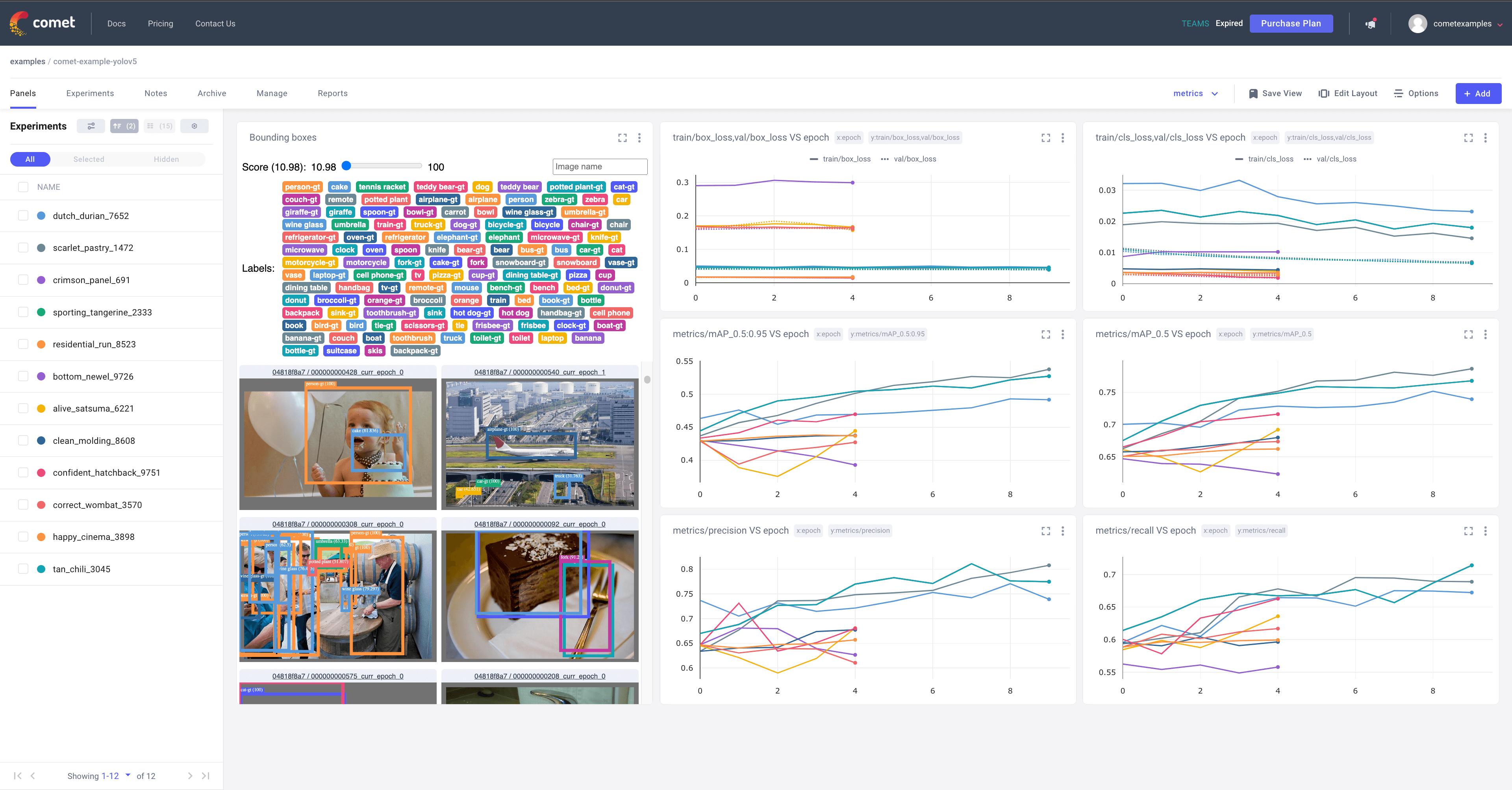
Logging Model Predictions

By default, model predictions (images, ground truth labels and bounding boxes) will be logged to Comet.

You can control the frequency of logged predictions and the associated images by passing the bbox_interval command line argument. Predictions can be visualized using Comet's Object Detection Custom Panel. This frequency corresponds to every Nth batch of data per epoch. In the example below, we are logging every 2nd batch of data for each epoch.

Note: The YOLOv5 validation dataloader will default to a batch size of 32, so you will have to set the logging frequency accordingly.

Here is an example project using the Panel

python train.py \
--img 640 \
--batch 16 \
--epochs 5 \
--data coco128.yaml \
--weights yolov5s.pt \
--bbox_interval 2

Controlling the number of Prediction Images logged to Comet

When logging predictions from YOLOv5, Comet will log the images associated with each set of predictions. By default a maximum of 100 validation images are logged. You can increase or decrease this number using the COMET_MAX_IMAGE_UPLOADS environment variable.

env COMET_MAX_IMAGE_UPLOADS=200 python train.py \
--img 640 \
--batch 16 \
--epochs 5 \
--data coco128.yaml \
--weights yolov5s.pt \
--bbox_interval 1

Logging Class Level Metrics

Use the COMET_LOG_PER_CLASS_METRICS environment variable to log mAP, precision, recall, f1 for each class.

env COMET_LOG_PER_CLASS_METRICS=true python train.py \
--img 640 \
--batch 16 \
--epochs 5 \
--data coco128.yaml \
--weights yolov5s.pt

Uploading a Dataset to Comet Artifacts

If you would like to store your data using Comet Artifacts, you can do so using the upload_dataset flag.

The dataset be organized in the way described in the YOLOv5 documentation. The dataset config yaml file must follow the same format as that of the coco128.yaml file.

python train.py \
--img 640 \
--batch 16 \
--epochs 5 \
--data coco128.yaml \
--weights yolov5s.pt \
--upload_dataset

You can find the uploaded dataset in the Artifacts tab in your Comet Workspace

You can preview the data directly in the Comet UI.

Artifacts are versioned and also support adding metadata about the dataset. Comet will automatically log the metadata from your dataset yaml file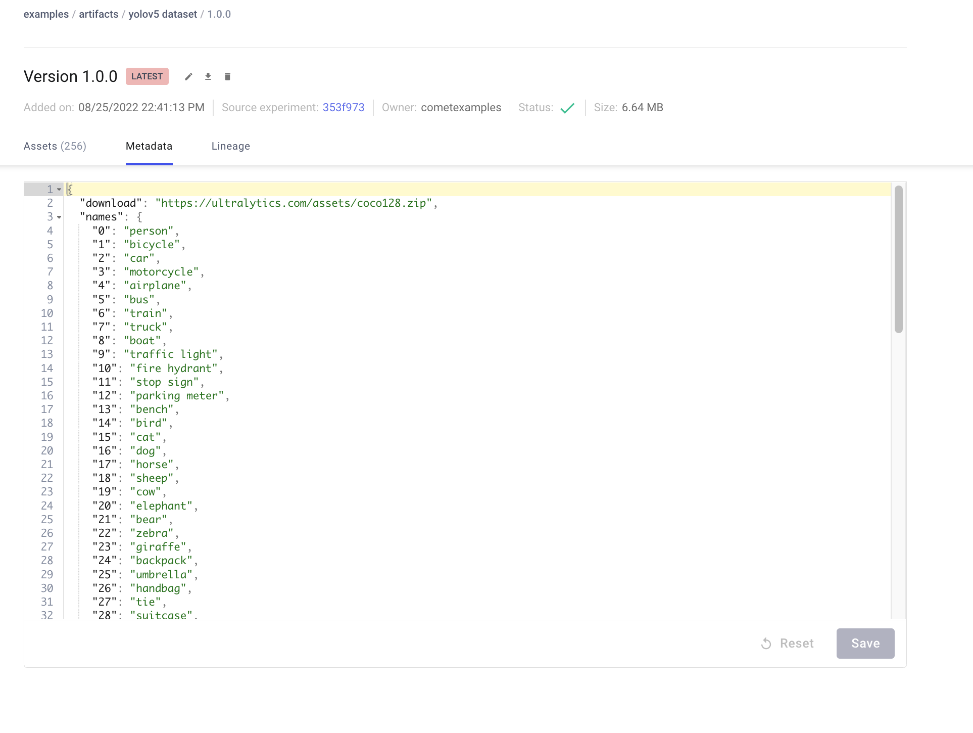

Using a saved Artifact

If you would like to use a dataset from Comet Artifacts, set the path variable in your dataset yaml file to point to the following Artifact resource URL.

# contents of artifact.yaml file
path: "comet://<workspace name>/<artifact name>:<artifact version or alias>"

Then pass this file to your training script in the following way

python train.py \
--img 640 \
--batch 16 \
--epochs 5 \
--data artifact.yaml \
--weights yolov5s.pt

Artifacts also allow you to track the lineage of data as it flows through your Experimentation workflow. Here you can see a graph that shows you all the experiments that have used your uploaded dataset.

Resuming a Training Run

If your training run is interrupted for any reason, e.g. disrupted internet connection, you can resume the run using the resume flag and the Comet Run Path.

The Run Path has the following format comet://<your workspace name>/<your project name>/<experiment id>.

This will restore the run to its state before the interruption, which includes restoring the model from a checkpoint, restoring all hyperparameters and training arguments and downloading Comet dataset Artifacts if they were used in the original run. The resumed run will continue logging to the existing Experiment in the Comet UI

python train.py \
--resume "comet://<your run path>"

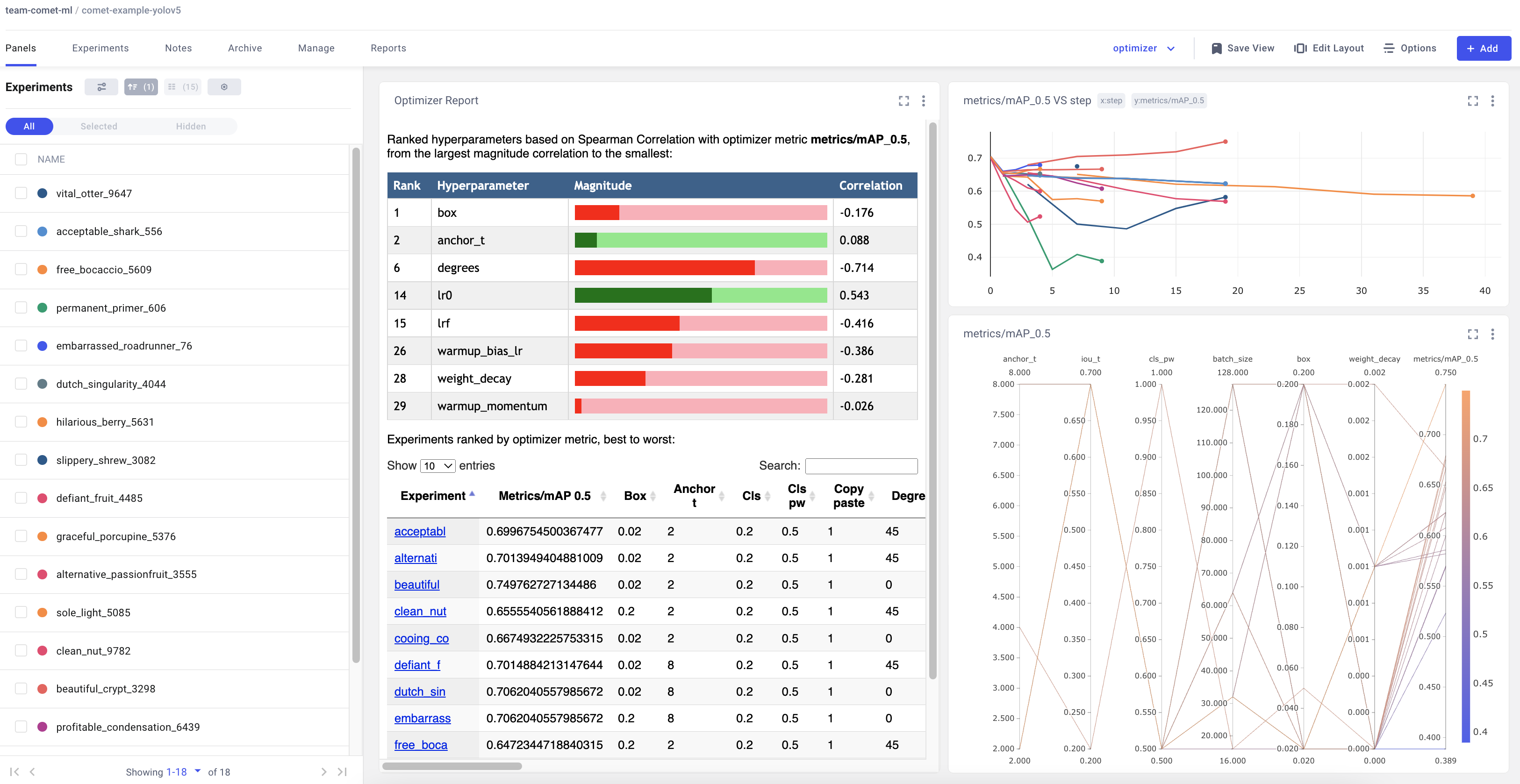
Hyperparameter Search with the Comet Optimizer

YOLOv5 is also integrated with Comet's Optimizer, making is simple to visualize hyperparameter sweeps in the Comet UI.

Configuring an Optimizer Sweep

To configure the Comet Optimizer, you will have to create a JSON file with the information about the sweep. An example file has been provided in utils/loggers/comet/optimizer_config.json

python utils/loggers/comet/hpo.py \
  --comet_optimizer_config "utils/loggers/comet/optimizer_config.json"

The hpo.py script accepts the same arguments as train.py. If you wish to pass additional arguments to your sweep simply add them after the script.

python utils/loggers/comet/hpo.py \
  --comet_optimizer_config "utils/loggers/comet/optimizer_config.json" \
  --save-period 1 \
  --bbox_interval 1

Running a Sweep in Parallel

comet optimizer -j <set number of workers> utils/loggers/comet/hpo.py \
  utils/loggers/comet/optimizer_config.json"

Visualizing Results

Comet provides a number of ways to visualize the results of your sweep. Take a look at a project with a completed sweep here

comments: true
description: Learn how to optimize YOLOv5 hyperparameters using genetic algorithms for improved training performance. Step-by-step instructions included.
keywords: YOLOv5, hyperparameter evolution, genetic algorithms, machine learning, optimization, Ultralytics

📚 This guide explains hyperparameter evolution for YOLOv5 🚀. Hyperparameter evolution is a method of Hyperparameter Optimization using a Genetic Algorithm (GA) for optimization.

Hyperparameters in ML control various aspects of training, and finding optimal values for them can be a challenge. Traditional methods like grid searches can quickly become intractable due to 1) the high dimensional search space 2) unknown correlations among the dimensions, and 3) expensive nature of evaluating the fitness at each point, making GA a suitable candidate for hyperparameter searches.

Before You Start

Clone repo and install requirements.txt in a Python>=3.8.0 environment, including PyTorch>=1.8. Models and datasets download automatically from the latest YOLOv5 release.

git clone https://github.com/ultralytics/yolov5  # clone
cd yolov5
pip install -r requirements.txt  # install

1. Initialize Hyperparameters

YOLOv5 has about 30 hyperparameters used for various training settings. These are defined in *.yaml files in the /data/hyps directory. Better initial guesses will produce better final results, so it is important to initialize these values properly before evolving. If in doubt, simply use the default values, which are optimized for YOLOv5 COCO training from scratch.

# YOLOv5 🚀 by Ultralytics, AGPL-3.0 license
# Hyperparameters for low-augmentation COCO training from scratch
# python train.py --batch 64 --cfg yolov5n6.yaml --weights '' --data coco.yaml --img 640 --epochs 300 --linear
# See tutorials for hyperparameter evolution https://github.com/ultralytics/yolov5#tutorials

lr0: 0.01 # initial learning rate (SGD=1E-2, Adam=1E-3)
lrf: 0.01 # final OneCycleLR learning rate (lr0 * lrf)
momentum: 0.937 # SGD momentum/Adam beta1
weight_decay: 0.0005 # optimizer weight decay 5e-4
warmup_epochs: 3.0 # warmup epochs (fractions ok)
warmup_momentum: 0.8 # warmup initial momentum
warmup_bias_lr: 0.1 # warmup initial bias lr
box: 0.05 # box loss gain
cls: 0.5 # cls loss gain
cls_pw: 1.0 # cls BCELoss positive_weight
obj: 1.0 # obj loss gain (scale with pixels)
obj_pw: 1.0 # obj BCELoss positive_weight
iou_t: 0.20 # IoU training threshold
anchor_t: 4.0 # anchor-multiple threshold
# anchors: 3  # anchors per output layer (0 to ignore)
fl_gamma: 0.0 # focal loss gamma (efficientDet default gamma=1.5)
hsv_h: 0.015 # image HSV-Hue augmentation (fraction)
hsv_s: 0.7 # image HSV-Saturation augmentation (fraction)
hsv_v: 0.4 # image HSV-Value augmentation (fraction)
degrees: 0.0 # image rotation (+/- deg)
translate: 0.1 # image translation (+/- fraction)
scale: 0.5 # image scale (+/- gain)
shear: 0.0 # image shear (+/- deg)
perspective: 0.0 # image perspective (+/- fraction), range 0-0.001
flipud: 0.0 # image flip up-down (probability)
fliplr: 0.5 # image flip left-right (probability)
mosaic: 1.0 # image mosaic (probability)
mixup: 0.0 # image mixup (probability)
copy_paste: 0.0 # segment copy-paste (probability)
```py

## 2. Define Fitness

Fitness is the value we seek to maximize. In YOLOv5 we define a default fitness function as a weighted combination of metrics: `mAP@0.5` contributes 10% of the weight and `mAP@0.5:0.95` contributes the remaining 90%, with [Precision `P` and Recall `R`](https://en.wikipedia.org/wiki/Precision_and_recall) absent. You may adjust these as you see fit or use the default fitness definition in utils/metrics.py (recommended).

```python
def fitness(x):
    """Return model fitness as the sum of weighted metrics [P, R, mAP@0.5, mAP@0.5:0.95]."""
    w = [0.0, 0.0, 0.1, 0.9]  # weights for [P, R, mAP@0.5, mAP@0.5:0.95]
    return (x[:, :4] * w).sum(1)
```py

## 3. Evolve

Evolution is performed about a base scenario which we seek to improve upon. The base scenario in this example is finetuning COCO128 for 10 epochs using pretrained YOLOv5s. The base scenario training command is:

```bash
python train.py --epochs 10 --data coco128.yaml --weights yolov5s.pt --cache
```py

To evolve hyperparameters **specific to this scenario**, starting from our initial values defined in **Section 1.**, and maximizing the fitness defined in **Section 2.**, append `--evolve`:

```bash
# Single-GPU
python train.py --epochs 10 --data coco128.yaml --weights yolov5s.pt --cache --evolve

# Multi-GPU
for i in 0 1 2 3 4 5 6 7; do
  sleep $(expr 30 \* $i) &&  # 30-second delay (optional)
  echo 'Starting GPU '$i'...' &&
  nohup python train.py --epochs 10 --data coco128.yaml --weights yolov5s.pt --cache --device $i --evolve > evolve_gpu_$i.log &
done

# Multi-GPU bash-while (not recommended)
for i in 0 1 2 3 4 5 6 7; do
  sleep $(expr 30 \* $i) &&  # 30-second delay (optional)
  echo 'Starting GPU '$i'...' &&
  "$(while true; do nohup python train.py... --device $i --evolve 1 > evolve_gpu_$i.log; done)" &
done
```py

The default evolution settings will run the base scenario 300 times, i.e. for 300 generations. You can modify generations via the `--evolve` argument, i.e. `python train.py --evolve 1000`.

The main genetic operators are **crossover** and **mutation**. In this work mutation is used, with an 80% probability and a 0.04 variance to create new offspring based on a combination of the best parents from all previous generations. Results are logged to `runs/evolve/exp/evolve.csv`, and the highest fitness offspring is saved every generation as `runs/evolve/hyp_evolved.yaml`:

```yaml
# YOLOv5 Hyperparameter Evolution Results
# Best generation: 287
# Last generation: 300
#    metrics/precision,       metrics/recall,      metrics/mAP_0.5, metrics/mAP_0.5:0.95,         val/box_loss,         val/obj_loss,         val/cls_loss
#              0.54634,              0.55625,              0.58201,              0.33665,             0.056451,             0.042892,             0.013441

lr0: 0.01 # initial learning rate (SGD=1E-2, Adam=1E-3)
lrf: 0.2 # final OneCycleLR learning rate (lr0 * lrf)
momentum: 0.937 # SGD momentum/Adam beta1
weight_decay: 0.0005 # optimizer weight decay 5e-4
warmup_epochs: 3.0 # warmup epochs (fractions ok)
warmup_momentum: 0.8 # warmup initial momentum
warmup_bias_lr: 0.1 # warmup initial bias lr
box: 0.05 # box loss gain
cls: 0.5 # cls loss gain
cls_pw: 1.0 # cls BCELoss positive_weight
obj: 1.0 # obj loss gain (scale with pixels)
obj_pw: 1.0 # obj BCELoss positive_weight
iou_t: 0.20 # IoU training threshold
anchor_t: 4.0 # anchor-multiple threshold
# anchors: 3  # anchors per output layer (0 to ignore)
fl_gamma: 0.0 # focal loss gamma (efficientDet default gamma=1.5)
hsv_h: 0.015 # image HSV-Hue augmentation (fraction)
hsv_s: 0.7 # image HSV-Saturation augmentation (fraction)
hsv_v: 0.4 # image HSV-Value augmentation (fraction)
degrees: 0.0 # image rotation (+/- deg)
translate: 0.1 # image translation (+/- fraction)
scale: 0.5 # image scale (+/- gain)
shear: 0.0 # image shear (+/- deg)
perspective: 0.0 # image perspective (+/- fraction), range 0-0.001
flipud: 0.0 # image flip up-down (probability)
fliplr: 0.5 # image flip left-right (probability)
mosaic: 1.0 # image mosaic (probability)
mixup: 0.0 # image mixup (probability)
copy_paste: 0.0 # segment copy-paste (probability)

We recommend a minimum of 300 generations of evolution for best results. Note that evolution is generally expensive and time-consuming, as the base scenario is trained hundreds of times, possibly requiring hundreds or thousands of GPU hours.

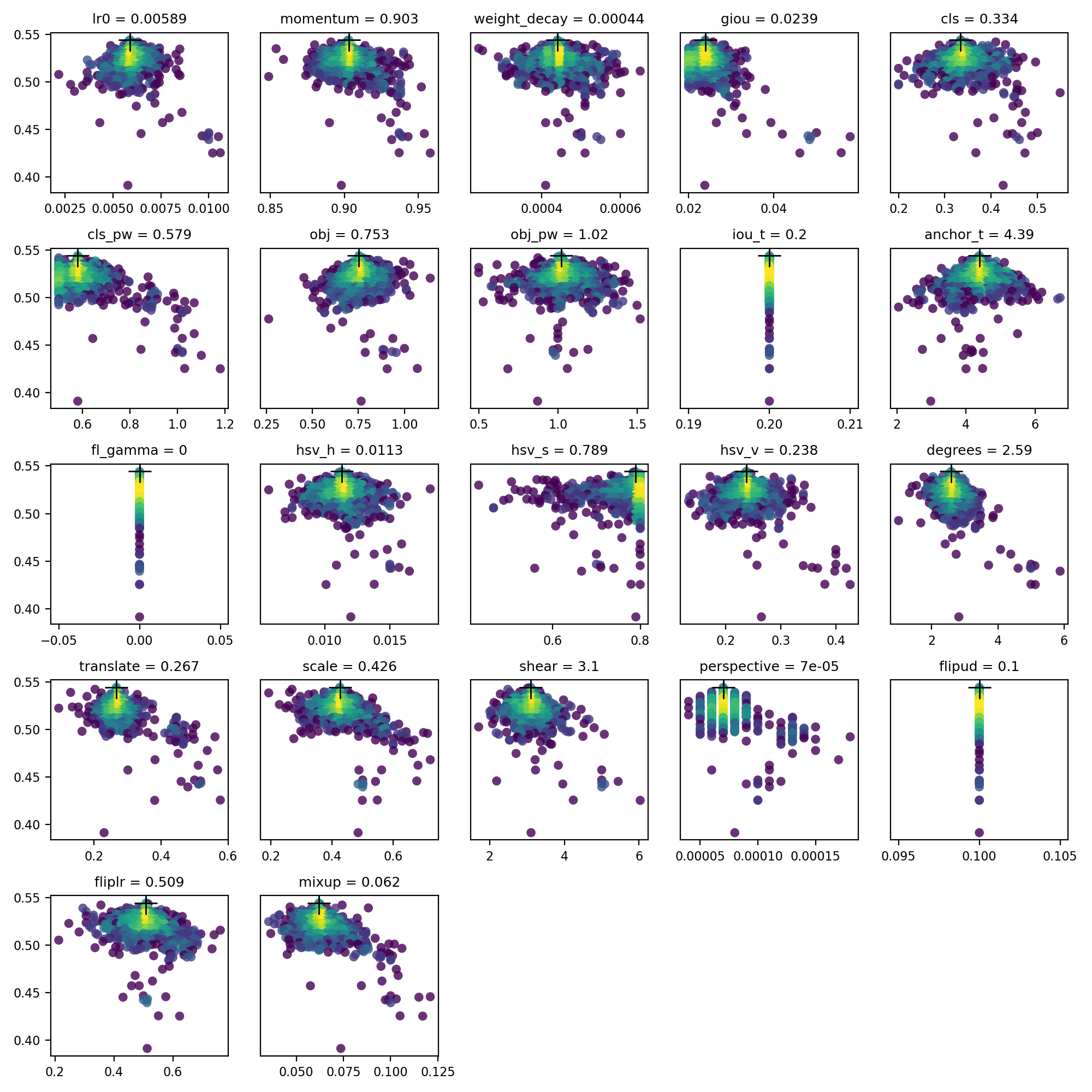
4. Visualize

evolve.csv is plotted as evolve.png by utils.plots.plot_evolve() after evolution finishes with one subplot per hyperparameter showing fitness (y-axis) vs hyperparameter values (x-axis). Yellow indicates higher concentrations. Vertical distributions indicate that a parameter has been disabled and does not mutate. This is user selectable in the meta dictionary in train.py, and is useful for fixing parameters and preventing them from evolving.

Supported Environments

Ultralytics provides a range of ready-to-use environments, each pre-installed with essential dependencies such as CUDA, CUDNN, Python, and PyTorch, to kickstart your projects.

Free GPU Notebooks:
Google Cloud: GCP Quickstart Guide
Amazon: AWS Quickstart Guide
Azure: AzureML Quickstart Guide
Docker: Docker Quickstart Guide

Project Status

comments: true
description: Learn how to use YOLOv5 model ensembling during testing and inference to enhance mAP and Recall for more accurate predictions.
keywords: YOLOv5, model ensembling, testing, inference, mAP, Recall, Ultralytics, object detection, PyTorch

📚 This guide explains how to use YOLOv5 🚀 model ensembling during testing and inference for improved mAP and Recall.

From https://en.wikipedia.org/wiki/Ensemble_learning:

Ensemble modeling is a process where multiple diverse models are created to predict an outcome, either by using many different modeling algorithms or using different training data sets. The ensemble model then aggregates the prediction of each base model and results in once final prediction for the unseen data. The motivation for using ensemble models is to reduce the generalization error of the prediction. As long as the base models are diverse and independent, the prediction error of the model decreases when the ensemble approach is used. The approach seeks the wisdom of crowds in making a prediction. Even though the ensemble model has multiple base models within the model, it acts and performs as a single model.

Before You Start

Clone repo and install requirements.txt in a Python>=3.8.0 environment, including PyTorch>=1.8. Models and datasets download automatically from the latest YOLOv5 release.

git clone https://github.com/ultralytics/yolov5  # clone
cd yolov5
pip install -r requirements.txt  # install

Test Normally

Before ensembling we want to establish the baseline performance of a single model. This command tests YOLOv5x on COCO val2017 at image size 640 pixels. yolov5x.pt is the largest and most accurate model available. Other options are yolov5s.pt, yolov5m.pt and yolov5l.pt, or you own checkpoint from training a custom dataset ./weights/best.pt. For details on all available models please see our README table.

python val.py --weights yolov5x.pt --data coco.yaml --img 640 --half

Output:

val: data=./data/coco.yaml, weights=['yolov5x.pt'], batch_size=32, imgsz=640, conf_thres=0.001, iou_thres=0.65, task=val, device=, single_cls=False, augment=False, verbose=False, save_txt=False, save_hybrid=False, save_conf=False, save_json=True, project=runs/val, name=exp, exist_ok=False, half=True
YOLOv5 🚀 v5.0-267-g6a3ee7c torch 1.9.0+cu102 CUDA:0 (Tesla P100-PCIE-16GB, 16280.875MB)

Fusing layers...
Model Summary: 476 layers, 87730285 parameters, 0 gradients

val: Scanning '../datasets/coco/val2017' images and labels...4952 found, 48 missing, 0 empty, 0 corrupted: 100% 5000/5000 [00:01<00:00, 2846.03it/s]
val: New cache created: ../datasets/coco/val2017.cache
               Class     Images     Labels          P          R     mAP@.5 mAP@.5:.95: 100% 157/157 [02:30<00:00,  1.05it/s]
                 all       5000      36335      0.746      0.626       0.68       0.49
Speed: 0.1ms pre-process, 22.4ms inference, 1.4ms NMS per image at shape (32, 3, 640, 640)  # <--- baseline speed

Evaluating pycocotools mAP... saving runs/val/exp/yolov5x_predictions.json...
...
 Average Precision  (AP) @[ IoU=0.50:0.95 | area=   all | maxDets=100 ] = 0.504  # <--- baseline mAP
 Average Precision  (AP) @[ IoU=0.50      | area=   all | maxDets=100 ] = 0.688
 Average Precision  (AP) @[ IoU=0.75      | area=   all | maxDets=100 ] = 0.546
 Average Precision  (AP) @[ IoU=0.50:0.95 | area= small | maxDets=100 ] = 0.351
 Average Precision  (AP) @[ IoU=0.50:0.95 | area=medium | maxDets=100 ] = 0.551
 Average Precision  (AP) @[ IoU=0.50:0.95 | area= large | maxDets=100 ] = 0.644
 Average Recall     (AR) @[ IoU=0.50:0.95 | area=   all | maxDets=  1 ] = 0.382
 Average Recall     (AR) @[ IoU=0.50:0.95 | area=   all | maxDets= 10 ] = 0.628
 Average Recall     (AR) @[ IoU=0.50:0.95 | area=   all | maxDets=100 ] = 0.681  # <--- baseline mAR
 Average Recall     (AR) @[ IoU=0.50:0.95 | area= small | maxDets=100 ] = 0.524
 Average Recall     (AR) @[ IoU=0.50:0.95 | area=medium | maxDets=100 ] = 0.735
 Average Recall     (AR) @[ IoU=0.50:0.95 | area= large | maxDets=100 ] = 0.826
```py

## Ensemble Test

Multiple pretrained models may be ensembled together at test and inference time by simply appending extra models to the `--weights` argument in any existing val.py or detect.py command. This example tests an ensemble of 2 models together:

- YOLOv5x
- YOLOv5l6

```bash
python val.py --weights yolov5x.pt yolov5l6.pt --data coco.yaml --img 640 --half
```py

Output:

```shell
val: data=./data/coco.yaml, weights=['yolov5x.pt', 'yolov5l6.pt'], batch_size=32, imgsz=640, conf_thres=0.001, iou_thres=0.6, task=val, device=, single_cls=False, augment=False, verbose=False, save_txt=False, save_hybrid=False, save_conf=False, save_json=True, project=runs/val, name=exp, exist_ok=False, half=True
YOLOv5 🚀 v5.0-267-g6a3ee7c torch 1.9.0+cu102 CUDA:0 (Tesla P100-PCIE-16GB, 16280.875MB)

Fusing layers...
Model Summary: 476 layers, 87730285 parameters, 0 gradients  # Model 1
Fusing layers...
Model Summary: 501 layers, 77218620 parameters, 0 gradients  # Model 2
Ensemble created with ['yolov5x.pt', 'yolov5l6.pt']  # Ensemble notice

val: Scanning '../datasets/coco/val2017.cache' images and labels... 4952 found, 48 missing, 0 empty, 0 corrupted: 100% 5000/5000 [00:00<00:00, 49695545.02it/s]
               Class     Images     Labels          P          R     mAP@.5 mAP@.5:.95: 100% 157/157 [03:58<00:00,  1.52s/it]
                 all       5000      36335      0.747      0.637      0.692      0.502
Speed: 0.1ms pre-process, 39.5ms inference, 2.0ms NMS per image at shape (32, 3, 640, 640)  # <--- ensemble speed

Evaluating pycocotools mAP... saving runs/val/exp3/yolov5x_predictions.json...
...
 Average Precision  (AP) @[ IoU=0.50:0.95 | area=   all | maxDets=100 ] = 0.515  # <--- ensemble mAP
 Average Precision  (AP) @[ IoU=0.50      | area=   all | maxDets=100 ] = 0.699
 Average Precision  (AP) @[ IoU=0.75      | area=   all | maxDets=100 ] = 0.557
 Average Precision  (AP) @[ IoU=0.50:0.95 | area= small | maxDets=100 ] = 0.356
 Average Precision  (AP) @[ IoU=0.50:0.95 | area=medium | maxDets=100 ] = 0.563
 Average Precision  (AP) @[ IoU=0.50:0.95 | area= large | maxDets=100 ] = 0.668
 Average Recall     (AR) @[ IoU=0.50:0.95 | area=   all | maxDets=  1 ] = 0.387
 Average Recall     (AR) @[ IoU=0.50:0.95 | area=   all | maxDets= 10 ] = 0.638
 Average Recall     (AR) @[ IoU=0.50:0.95 | area=   all | maxDets=100 ] = 0.689  # <--- ensemble mAR
 Average Recall     (AR) @[ IoU=0.50:0.95 | area= small | maxDets=100 ] = 0.526
 Average Recall     (AR) @[ IoU=0.50:0.95 | area=medium | maxDets=100 ] = 0.743
 Average Recall     (AR) @[ IoU=0.50:0.95 | area= large | maxDets=100 ] = 0.844
```py

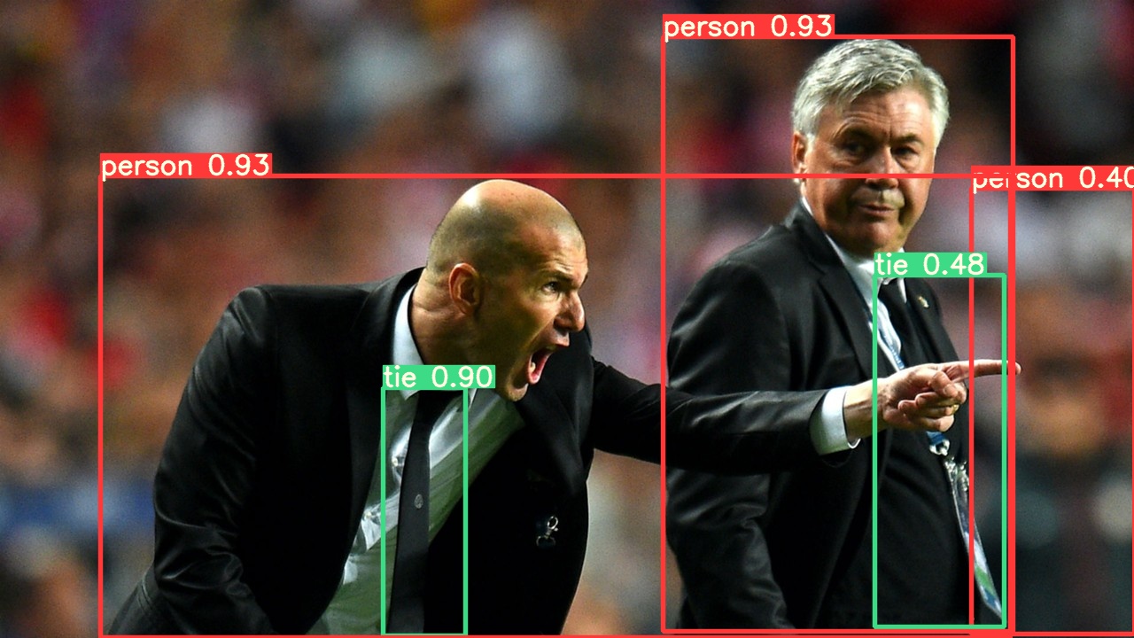
## Ensemble Inference

Append extra models to the `--weights` argument to run ensemble inference:

```bash
python detect.py --weights yolov5x.pt yolov5l6.pt --img 640 --source data/images
```py

Output:

```bash
YOLOv5 🚀 v5.0-267-g6a3ee7c torch 1.9.0+cu102 CUDA:0 (Tesla P100-PCIE-16GB, 16280.875MB)

Fusing layers...
Model Summary: 476 layers, 87730285 parameters, 0 gradients
Fusing layers...
Model Summary: 501 layers, 77218620 parameters, 0 gradients
Ensemble created with ['yolov5x.pt', 'yolov5l6.pt']

image 1/2 /content/yolov5/data/images/bus.jpg: 640x512 4 persons, 1 bus, 1 tie, Done. (0.063s)
image 2/2 /content/yolov5/data/images/zidane.jpg: 384x640 3 persons, 2 ties, Done. (0.056s)
Results saved to runs/detect/exp2
Done. (0.223s)

Supported Environments

Ultralytics provides a range of ready-to-use environments, each pre-installed with essential dependencies such as CUDA, CUDNN, Python, and PyTorch, to kickstart your projects.

Free GPU Notebooks:
Google Cloud: GCP Quickstart Guide
Amazon: AWS Quickstart Guide
Azure: AzureML Quickstart Guide
Docker: Docker Quickstart Guide

Project Status

comments: true
description: Learn to export YOLOv5 models to various formats like TFLite, ONNX, CoreML and TensorRT. Increase model efficiency and deployment flexibility with our step-by-step guide.
keywords: YOLOv5 export, TFLite, ONNX, CoreML, TensorRT, model conversion, YOLOv5 tutorial, PyTorch export

TFLite, ONNX, CoreML, TensorRT Export

📚 This guide explains how to export a trained YOLOv5 🚀 model from PyTorch to ONNX and TorchScript formats.

Before You Start

Clone repo and install requirements.txt in a Python>=3.8.0 environment, including PyTorch>=1.8. Models and datasets download automatically from the latest YOLOv5 release.

git clone https://github.com/ultralytics/yolov5  # clone
cd yolov5
pip install -r requirements.txt  # install

For TensorRT export example (requires GPU) see our Colab notebook appendix section.

Formats

YOLOv5 inference is officially supported in 11 formats:

💡 ProTip: Export to ONNX or OpenVINO for up to 3x CPU speedup. See CPU Benchmarks. 💡 ProTip: Export to TensorRT for up to 5x GPU speedup. See GPU Benchmarks.

Format	`export.py --include`	Model
PyTorch	-	`yolov5s.pt`
TorchScript	`torchscript`	`yolov5s.torchscript`
ONNX	`onnx`	`yolov5s.onnx`
OpenVINO	`openvino`	`yolov5s_openvino_model/`
TensorRT	`engine`	`yolov5s.engine`
CoreML	`coreml`	`yolov5s.mlmodel`
TensorFlow SavedModel	`saved_model`	`yolov5s_saved_model/`
TensorFlow GraphDef	`pb`	`yolov5s.pb`
TensorFlow Lite	`tflite`	`yolov5s.tflite`
TensorFlow Edge TPU	`edgetpu`	`yolov5s_edgetpu.tflite`
TensorFlow.js	`tfjs`	`yolov5s_web_model/`
PaddlePaddle	`paddle`	`yolov5s_paddle_model/`

Benchmarks

Benchmarks below run on a Colab Pro with the YOLOv5 tutorial notebook . To reproduce:

python benchmarks.py --weights yolov5s.pt --imgsz 640 --device 0

Colab Pro V100 GPU

benchmarks: weights=/content/yolov5/yolov5s.pt, imgsz=640, batch_size=1, data=/content/yolov5/data/coco128.yaml, device=0, half=False, test=False
Checking setup...
YOLOv5 🚀 v6.1-135-g7926afc torch 1.10.0+cu111 CUDA:0 (Tesla V100-SXM2-16GB, 16160MiB)
Setup complete ✅ (8 CPUs, 51.0 GB RAM, 46.7/166.8 GB disk)

Benchmarks complete (458.07s)
                   Format  mAP@0.5:0.95  Inference time (ms)
0                 PyTorch        0.4623                10.19
1             TorchScript        0.4623                 6.85
2                    ONNX        0.4623                14.63
3                OpenVINO           NaN                  NaN
4                TensorRT        0.4617                 1.89
5                  CoreML           NaN                  NaN
6   TensorFlow SavedModel        0.4623                21.28
7     TensorFlow GraphDef        0.4623                21.22
8         TensorFlow Lite           NaN                  NaN
9     TensorFlow Edge TPU           NaN                  NaN
10          TensorFlow.js           NaN                  NaN
```py

### Colab Pro CPU

benchmarks: weights=/content/yolov5/yolov5s.pt, imgsz=640, batch_size=1, data=/content/yolov5/data/coco128.yaml, device=cpu, half=False, test=False
Checking setup...
YOLOv5 🚀 v6.1-135-g7926afc torch 1.10.0+cu111 CPU
Setup complete ✅ (8 CPUs, 51.0 GB RAM, 41.5/166.8 GB disk)

Benchmarks complete (241.20s)
Format mAP@0.5:0.95 Inference time (ms)
0 PyTorch 0.4623 127.61
1 TorchScript 0.4623 131.23
2 ONNX 0.4623 69.34
3 OpenVINO 0.4623 66.52
4 TensorRT NaN NaN
5 CoreML NaN NaN
6 TensorFlow SavedModel 0.4623 123.79
7 TensorFlow GraphDef 0.4623 121.57
8 TensorFlow Lite 0.4623 316.61
9 TensorFlow Edge TPU NaN NaN
10 TensorFlow.js NaN NaN


## Export a Trained YOLOv5 Model

This command exports a pretrained YOLOv5s model to TorchScript and ONNX formats. `yolov5s.pt` is the 'small' model, the second-smallest model available. Other options are `yolov5n.pt`, `yolov5m.pt`, `yolov5l.pt` and `yolov5x.pt`, along with their P6 counterparts i.e. `yolov5s6.pt` or you own custom training checkpoint i.e. `runs/exp/weights/best.pt`. For details on all available models please see our README [table](https://github.com/ultralytics/yolov5#pretrained-checkpoints).

```bash
python export.py --weights yolov5s.pt --include torchscript onnx

💡 ProTip: Add --half to export models at FP16 half precision for smaller file sizes

Output:

export: data=data/coco128.yaml, weights=['yolov5s.pt'], imgsz=[640, 640], batch_size=1, device=cpu, half=False, inplace=False, train=False, keras=False, optimize=False, int8=False, dynamic=False, simplify=False, opset=12, verbose=False, workspace=4, nms=False, agnostic_nms=False, topk_per_class=100, topk_all=100, iou_thres=0.45, conf_thres=0.25, include=['torchscript', 'onnx']
YOLOv5 🚀 v6.2-104-ge3e5122 Python-3.8.0 torch-1.12.1+cu113 CPU

Downloading https://github.com/ultralytics/yolov5/releases/download/v6.2/yolov5s.pt to yolov5s.pt...
100% 14.1M/14.1M [00:00<00:00, 274MB/s]

Fusing layers...
YOLOv5s summary: 213 layers, 7225885 parameters, 0 gradients

PyTorch: starting from yolov5s.pt with output shape (1, 25200, 85) (14.1 MB)

TorchScript: starting export with torch 1.12.1+cu113...
TorchScript: export success ✅ 1.7s, saved as yolov5s.torchscript (28.1 MB)

ONNX: starting export with onnx 1.12.0...
ONNX: export success ✅ 2.3s, saved as yolov5s.onnx (28.0 MB)

Export complete (5.5s)
Results saved to /content/yolov5
Detect:          python detect.py --weights yolov5s.onnx
Validate:        python val.py --weights yolov5s.onnx
PyTorch Hub:     model = torch.hub.load('ultralytics/yolov5', 'custom', 'yolov5s.onnx')
Visualize:       https://netron.app/
```py

The 3 exported models will be saved alongside the original PyTorch model:

<p align="center"><img width="700" src="https://user-images.githubusercontent.com/26833433/122827190-57a8f880-d2e4-11eb-860e-dbb7f9fc57fb.png" alt="YOLO export locations"></p>

[Netron Viewer](https://github.com/lutzroeder/netron) is recommended for visualizing exported models:

<p align="center"><img width="850" src="https://user-images.githubusercontent.com/26833433/191003260-f94011a7-5b2e-4fe3-93c1-e1a935e0a728.png" alt="YOLO model visualization"></p>

## Exported Model Usage Examples

`detect.py` runs inference on exported models:

```bash
python detect.py --weights yolov5s.pt                 # PyTorch
                           yolov5s.torchscript        # TorchScript
                           yolov5s.onnx               # ONNX Runtime or OpenCV DNN with dnn=True
                           yolov5s_openvino_model     # OpenVINO
                           yolov5s.engine             # TensorRT
                           yolov5s.mlmodel            # CoreML (macOS only)
                           yolov5s_saved_model        # TensorFlow SavedModel
                           yolov5s.pb                 # TensorFlow GraphDef
                           yolov5s.tflite             # TensorFlow Lite
                           yolov5s_edgetpu.tflite     # TensorFlow Edge TPU
                           yolov5s_paddle_model       # PaddlePaddle
```py

`val.py` runs validation on exported models:

```bash
python val.py --weights yolov5s.pt                 # PyTorch
                        yolov5s.torchscript        # TorchScript
                        yolov5s.onnx               # ONNX Runtime or OpenCV DNN with dnn=True
                        yolov5s_openvino_model     # OpenVINO
                        yolov5s.engine             # TensorRT
                        yolov5s.mlmodel            # CoreML (macOS Only)
                        yolov5s_saved_model        # TensorFlow SavedModel
                        yolov5s.pb                 # TensorFlow GraphDef
                        yolov5s.tflite             # TensorFlow Lite
                        yolov5s_edgetpu.tflite     # TensorFlow Edge TPU
                        yolov5s_paddle_model       # PaddlePaddle
```py

Use PyTorch Hub with exported YOLOv5 models:

```python
import torch

# Model
model = torch.hub.load("ultralytics/yolov5", "custom", "yolov5s.pt")
model = torch.hub.load("ultralytics/yolov5", "custom", "yolov5s.torchscript ")  # TorchScript
model = torch.hub.load("ultralytics/yolov5", "custom", "yolov5s.onnx")  # ONNX Runtime
model = torch.hub.load("ultralytics/yolov5", "custom", "yolov5s_openvino_model")  # OpenVINO
model = torch.hub.load("ultralytics/yolov5", "custom", "yolov5s.engine")  # TensorRT
model = torch.hub.load("ultralytics/yolov5", "custom", "yolov5s.mlmodel")  # CoreML (macOS Only)
model = torch.hub.load("ultralytics/yolov5", "custom", "yolov5s_saved_model")  # TensorFlow SavedModel
model = torch.hub.load("ultralytics/yolov5", "custom", "yolov5s.pb")  # TensorFlow GraphDef
model = torch.hub.load("ultralytics/yolov5", "custom", "yolov5s.tflite")  # TensorFlow Lite
model = torch.hub.load("ultralytics/yolov5", "custom", "yolov5s_edgetpu.tflite")  # TensorFlow Edge TPU
model = torch.hub.load("ultralytics/yolov5", "custom", "yolov5s_paddle_model")  # PaddlePaddle

# Images
img = "https://ultralytics.com/images/zidane.jpg"  # or file, Path, PIL, OpenCV, numpy, list

# Inference
results = model(img)

# Results
results.print()  # or .show(), .save(), .crop(), .pandas(), etc.
```py

## OpenCV DNN inference

OpenCV inference with ONNX models:

```bash
python export.py --weights yolov5s.pt --include onnx

python detect.py --weights yolov5s.onnx --dnn  # detect
python val.py --weights yolov5s.onnx --dnn  # validate

C++ Inference

YOLOv5 OpenCV DNN C++ inference on exported ONNX model examples:

YOLOv5 OpenVINO C++ inference examples:

TensorFlow.js Web Browser Inference

https://aukerul-shuvo.github.io/YOLOv5_TensorFlow-JS/

Supported Environments

Ultralytics provides a range of ready-to-use environments, each pre-installed with essential dependencies such as CUDA, CUDNN, Python, and PyTorch, to kickstart your projects.

Free GPU Notebooks:
Google Cloud: GCP Quickstart Guide
Amazon: AWS Quickstart Guide
Azure: AzureML Quickstart Guide
Docker: Docker Quickstart Guide

Project Status

comments: true
description: Learn how to prune YOLOv5 models for improved performance. Follow this step-by-step guide to optimize your YOLOv5 models effectively.
keywords: YOLOv5 pruning, model pruning, YOLOv5 optimization, YOLOv5 guide, machine learning pruning

📚 This guide explains how to apply pruning to YOLOv5 🚀 models.

Before You Start

Clone repo and install requirements.txt in a Python>=3.8.0 environment, including PyTorch>=1.8. Models and datasets download automatically from the latest YOLOv5 release.

git clone https://github.com/ultralytics/yolov5  # clone
cd yolov5
pip install -r requirements.txt  # install

Test Normally

Before pruning we want to establish a baseline performance to compare to. This command tests YOLOv5x on COCO val2017 at image size 640 pixels. yolov5x.pt is the largest and most accurate model available. Other options are yolov5s.pt, yolov5m.pt and yolov5l.pt, or you own checkpoint from training a custom dataset ./weights/best.pt. For details on all available models please see our README table.

python val.py --weights yolov5x.pt --data coco.yaml --img 640 --half

Output:

val: data=/content/yolov5/data/coco.yaml, weights=['yolov5x.pt'], batch_size=32, imgsz=640, conf_thres=0.001, iou_thres=0.65, task=val, device=, workers=8, single_cls=False, augment=False, verbose=False, save_txt=False, save_hybrid=False, save_conf=False, save_json=True, project=runs/val, name=exp, exist_ok=False, half=True, dnn=False
YOLOv5 🚀 v6.0-224-g4c40933 torch 1.10.0+cu111 CUDA:0 (Tesla V100-SXM2-16GB, 16160MiB)

Fusing layers...
Model Summary: 444 layers, 86705005 parameters, 0 gradients
val: Scanning '/content/datasets/coco/val2017.cache' images and labels... 4952 found, 48 missing, 0 empty, 0 corrupt: 100% 5000/5000 [00:00<?, ?it/s]
               Class     Images     Labels          P          R     mAP@.5 mAP@.5:.95: 100% 157/157 [01:12<00:00,  2.16it/s]
                 all       5000      36335      0.732      0.628      0.683      0.496
Speed: 0.1ms pre-process, 5.2ms inference, 1.7ms NMS per image at shape (32, 3, 640, 640)  # <--- base speed

Evaluating pycocotools mAP... saving runs/val/exp2/yolov5x_predictions.json...
...
 Average Precision  (AP) @[ IoU=0.50:0.95 | area=   all | maxDets=100 ] = 0.507  # <--- base mAP
 Average Precision  (AP) @[ IoU=0.50      | area=   all | maxDets=100 ] = 0.689
 Average Precision  (AP) @[ IoU=0.75      | area=   all | maxDets=100 ] = 0.552
 Average Precision  (AP) @[ IoU=0.50:0.95 | area= small | maxDets=100 ] = 0.345
 Average Precision  (AP) @[ IoU=0.50:0.95 | area=medium | maxDets=100 ] = 0.559
 Average Precision  (AP) @[ IoU=0.50:0.95 | area= large | maxDets=100 ] = 0.652
 Average Recall     (AR) @[ IoU=0.50:0.95 | area=   all | maxDets=  1 ] = 0.381
 Average Recall     (AR) @[ IoU=0.50:0.95 | area=   all | maxDets= 10 ] = 0.630
 Average Recall     (AR) @[ IoU=0.50:0.95 | area=   all | maxDets=100 ] = 0.682
 Average Recall     (AR) @[ IoU=0.50:0.95 | area= small | maxDets=100 ] = 0.526
 Average Recall     (AR) @[ IoU=0.50:0.95 | area=medium | maxDets=100 ] = 0.731
 Average Recall     (AR) @[ IoU=0.50:0.95 | area= large | maxDets=100 ] = 0.829
Results saved to runs/val/exp
```py

## Test YOLOv5x on COCO (0.30 sparsity)

We repeat the above test with a pruned model by using the `torch_utils.prune()` command. We update `val.py` to prune YOLOv5x to 0.3 sparsity:

<img width="894" alt="Screenshot 2022-02-02 at 22 54 18" src="https://user-images.githubusercontent.com/26833433/152243799-b0ac2777-b1a8-47b1-801a-2e4c93c06ead.png">

30% pruned output:

```bash
val: data=/content/yolov5/data/coco.yaml, weights=['yolov5x.pt'], batch_size=32, imgsz=640, conf_thres=0.001, iou_thres=0.65, task=val, device=, workers=8, single_cls=False, augment=False, verbose=False, save_txt=False, save_hybrid=False, save_conf=False, save_json=True, project=runs/val, name=exp, exist_ok=False, half=True, dnn=False
YOLOv5 🚀 v6.0-224-g4c40933 torch 1.10.0+cu111 CUDA:0 (Tesla V100-SXM2-16GB, 16160MiB)

Fusing layers...
Model Summary: 444 layers, 86705005 parameters, 0 gradients
Pruning model...  0.3 global sparsity
val: Scanning '/content/datasets/coco/val2017.cache' images and labels... 4952 found, 48 missing, 0 empty, 0 corrupt: 100% 5000/5000 [00:00<?, ?it/s]
               Class     Images     Labels          P          R     mAP@.5 mAP@.5:.95: 100% 157/157 [01:11<00:00,  2.19it/s]
                 all       5000      36335      0.724      0.614      0.671      0.478
Speed: 0.1ms pre-process, 5.2ms inference, 1.7ms NMS per image at shape (32, 3, 640, 640)  # <--- prune mAP

Evaluating pycocotools mAP... saving runs/val/exp3/yolov5x_predictions.json...
...
 Average Precision  (AP) @[ IoU=0.50:0.95 | area=   all | maxDets=100 ] = 0.489  # <--- prune mAP
 Average Precision  (AP) @[ IoU=0.50      | area=   all | maxDets=100 ] = 0.677
 Average Precision  (AP) @[ IoU=0.75      | area=   all | maxDets=100 ] = 0.537
 Average Precision  (AP) @[ IoU=0.50:0.95 | area= small | maxDets=100 ] = 0.334
 Average Precision  (AP) @[ IoU=0.50:0.95 | area=medium | maxDets=100 ] = 0.542
 Average Precision  (AP) @[ IoU=0.50:0.95 | area= large | maxDets=100 ] = 0.635
 Average Recall     (AR) @[ IoU=0.50:0.95 | area=   all | maxDets=  1 ] = 0.370
 Average Recall     (AR) @[ IoU=0.50:0.95 | area=   all | maxDets= 10 ] = 0.612
 Average Recall     (AR) @[ IoU=0.50:0.95 | area=   all | maxDets=100 ] = 0.664
 Average Recall     (AR) @[ IoU=0.50:0.95 | area= small | maxDets=100 ] = 0.496
 Average Recall     (AR) @[ IoU=0.50:0.95 | area=medium | maxDets=100 ] = 0.722
 Average Recall     (AR) @[ IoU=0.50:0.95 | area= large | maxDets=100 ] = 0.803
Results saved to runs/val/exp3

In the results we can observe that we have achieved a sparsity of 30% in our model after pruning, which means that 30% of the model's weight parameters in nn.Conv2d layers are equal to 0. Inference time is essentially unchanged, while the model's AP and AR scores a slightly reduced.

Supported Environments

Ultralytics provides a range of ready-to-use environments, each pre-installed with essential dependencies such as CUDA, CUDNN, Python, and PyTorch, to kickstart your projects.

Free GPU Notebooks:
Google Cloud: GCP Quickstart Guide
Amazon: AWS Quickstart Guide
Azure: AzureML Quickstart Guide
Docker: Docker Quickstart Guide

Project Status

comments: true
description: Learn how to train YOLOv5 on multiple GPUs for optimal performance. Guide covers single and multiple machine setups.
keywords: YOLOv5, multiple GPUs, machine learning, deep learning, PyTorch, data parallel, distributed data parallel

📚 This guide explains how to properly use multiple GPUs to train a dataset with YOLOv5 🚀 on single or multiple machine(s).

Before You Start

Clone repo and install requirements.txt in a Python>=3.8.0 environment, including PyTorch>=1.8. Models and datasets download automatically from the latest YOLOv5 release.

git clone https://github.com/ultralytics/yolov5  # clone
cd yolov5
pip install -r requirements.txt  # install

💡 ProTip! Docker Image is recommended for all Multi-GPU trainings. See Docker Quickstart Guide

💡 ProTip! torch.distributed.run replaces torch.distributed.launch in PyTorch>=1.9. See docs for details.

Training

Select a pretrained model to start training from. Here we select YOLOv5s, the smallest and fastest model available. See our README table for a full comparison of all models. We will train this model with Multi-GPU on the COCO dataset.

Single GPU

python train.py  --batch 64 --data coco.yaml --weights yolov5s.pt --device 0

Multi-GPU DataParallel Mode (⚠️ not recommended)

You can increase the device to use Multiple GPUs in DataParallel mode.

python train.py  --batch 64 --data coco.yaml --weights yolov5s.pt --device 0,1

This method is slow and barely speeds up training compared to using just 1 GPU.

Multi-GPU DistributedDataParallel Mode (✅ recommended)

You will have to pass python -m torch.distributed.run --nproc_per_node, followed by the usual arguments.

python -m torch.distributed.run --nproc_per_node 2 train.py --batch 64 --data coco.yaml --weights yolov5s.pt --device 0,1

--nproc_per_node specifies how many GPUs you would like to use. In the example above, it is 2.
--batch is the total batch-size. It will be divided evenly to each GPU. In the example above, it is 64/2=32 per GPU.

The code above will use GPUs 0... (N-1).

Use specific GPUs (click to expand)

You can do so by simply passing --device followed by your specific GPUs. For example, in the code below, we will use GPUs 2,3.

python -m torch.distributed.run --nproc_per_node 2 train.py --batch 64 --data coco.yaml --cfg yolov5s.yaml --weights '' --device 2,3

Use SyncBatchNorm (click to expand)

SyncBatchNorm could increase accuracy for multiple gpu training, however, it will slow down training by a significant factor. It is only available for Multiple GPU DistributedDataParallel training.

It is best used when the batch-size on each GPU is small (<= 8).

To use SyncBatchNorm, simple pass --sync-bn to the command like below,

python -m torch.distributed.run --nproc_per_node 2 train.py --batch 64 --data coco.yaml --cfg yolov5s.yaml --weights '' --sync-bn

Use Multiple machines (click to expand)

This is only available for Multiple GPU DistributedDataParallel training.

Before we continue, make sure the files on all machines are the same, dataset, codebase, etc. Afterward, make sure the machines can communicate to each other.

You will have to choose a master machine(the machine that the others will talk to). Note down its address(master_addr) and choose a port(master_port). I will use master_addr = 192.168.1.1 and master_port = 1234 for the example below.

To use it, you can do as the following,

# On master machine 0
python -m torch.distributed.run --nproc_per_node G --nnodes N --node_rank 0 --master_addr "192.168.1.1" --master_port 1234 train.py --batch 64 --data coco.yaml --cfg yolov5s.yaml --weights ''

# On machine R
python -m torch.distributed.run --nproc_per_node G --nnodes N --node_rank R --master_addr "192.168.1.1" --master_port 1234 train.py --batch 64 --data coco.yaml --cfg yolov5s.yaml --weights ''

where G is number of GPU per machine, N is the number of machines, and R is the machine number from 0...(N-1). Let's say I have two machines with two GPUs each, it would be G = 2 , N = 2, and R = 1 for the above.

Training will not start until all N machines are connected. Output will only be shown on master machine!

Notes

Windows support is untested, Linux is recommended.
--batch must be a multiple of the number of GPUs.
GPU 0 will take slightly more memory than the other GPUs as it maintains EMA and is responsible for checkpointing etc.
If you get RuntimeError: Address already in use, it could be because you are running multiple trainings at a time. To fix this, simply use a different port number by adding --master_port like below,

python -m torch.distributed.run --master_port 1234 --nproc_per_node 2 ...

Results

DDP profiling results on an AWS EC2 P4d instance with 8x A100 SXM4-40GB for YOLOv5l for 1 COCO epoch.

Profiling code

# prepare
t=ultralytics/yolov5:latest && sudo docker pull $t && sudo docker run -it --ipc=host --gpus all -v "$(pwd)"/coco:/usr/src/coco $t
pip3 install torch==1.9.0+cu111 torchvision==0.10.0+cu111 -f https://download.pytorch.org/whl/torch_stable.html
cd .. && rm -rf app && git clone https://github.com/ultralytics/yolov5 -b master app && cd app
cp data/coco.yaml data/coco_profile.yaml

# profile
python train.py --batch-size 16 --data coco_profile.yaml --weights yolov5l.pt --epochs 1 --device 0
python -m torch.distributed.run --nproc_per_node 2 train.py --batch-size 32 --data coco_profile.yaml --weights yolov5l.pt --epochs 1 --device 0,1
python -m torch.distributed.run --nproc_per_node 4 train.py --batch-size 64 --data coco_profile.yaml --weights yolov5l.pt --epochs 1 --device 0,1,2,3
python -m torch.distributed.run --nproc_per_node 8 train.py --batch-size 128 --data coco_profile.yaml --weights yolov5l.pt --epochs 1 --device 0,1,2,3,4,5,6,7

GPUs A100	batch-size	CUDA_mem ^{device0 (G)}	COCO ^train	COCO ^val
1x	16	26GB	20:39	0:55
2x	32	26GB	11:43	0:57
4x	64	26GB	5:57	0:55
8x	128	26GB	3:09	0:57

FAQ

If an error occurs, please read the checklist below first! (It could save your time)

Checklist (click to expand)

Have you properly read this post?
Have you tried to re-clone the codebase? The code changes daily.
Have you tried to search for your error? Someone may have already encountered it in this repo or in another and have the solution.
Have you installed all the requirements listed on top (including the correct Python and Pytorch versions)?
Have you tried in other environments listed in the "Environments" section below?
Have you tried with another dataset like coco128 or coco2017? It will make it easier to find the root cause.

If you went through all the above, feel free to raise an Issue by giving as much detail as possible following the template.

Supported Environments

Ultralytics provides a range of ready-to-use environments, each pre-installed with essential dependencies such as CUDA, CUDNN, Python, and PyTorch, to kickstart your projects.

Free GPU Notebooks:
Google Cloud: GCP Quickstart Guide
Amazon: AWS Quickstart Guide
Azure: AzureML Quickstart Guide
Docker: Docker Quickstart Guide

Project Status

Credits

We would like to thank @MagicFrogSJTU, who did all the heavy lifting, and @glenn-jocher for guiding us along the way.

comments: true
description: Learn how to deploy YOLOv5 using Neural Magic's DeepSparse for GPU-class performance on CPUs. Discover easy integration, flexible deployments, and more.
keywords: YOLOv5, DeepSparse, Neural Magic, YOLO deployment, Sparse inference, Deep learning, Model sparsity, CPU optimization, No hardware accelerators, AI deployment

Welcome to software-delivered AI.

This guide explains how to deploy YOLOv5 with Neural Magic's DeepSparse.

DeepSparse is an inference runtime with exceptional performance on CPUs. For instance, compared to the ONNX Runtime baseline, DeepSparse offers a 5.8x speed-up for YOLOv5s, running on the same machine!

For the first time, your deep learning workloads can meet the performance demands of production without the complexity and costs of hardware accelerators. Put simply, DeepSparse gives you the performance of GPUs and the simplicity of software:

Flexible Deployments: Run consistently across cloud, data center, and edge with any hardware provider from Intel to AMD to ARM
Infinite Scalability: Scale vertically to 100s of cores, out with standard Kubernetes, or fully-abstracted with Serverless
Easy Integration: Clean APIs for integrating your model into an application and monitoring it in production

How Does DeepSparse Achieve GPU-Class Performance?

DeepSparse takes advantage of model sparsity to gain its performance speedup.

Sparsification through pruning and quantization is a broadly studied technique, allowing order-of-magnitude reductions in the size and compute needed to execute a network, while maintaining high accuracy. DeepSparse is sparsity-aware, meaning it skips the zeroed out parameters, shrinking amount of compute in a forward pass. Since the sparse computation is now memory bound, DeepSparse executes the network depth-wise, breaking the problem into Tensor Columns, vertical stripes of computation that fit in cache.

Sparse networks with compressed computation, executed depth-wise in cache, allows DeepSparse to deliver GPU-class performance on CPUs!

How Do I Create A Sparse Version of YOLOv5 Trained on My Data?

Neural Magic's open-source model repository, SparseZoo, contains pre-sparsified checkpoints of each YOLOv5 model. Using SparseML, which is integrated with Ultralytics, you can fine-tune a sparse checkpoint onto your data with a single CLI command.

Checkout Neural Magic's YOLOv5 documentation for more details.

DeepSparse Usage

We will walk through an example benchmarking and deploying a sparse version of YOLOv5s with DeepSparse.

Install DeepSparse

Run the following to install DeepSparse. We recommend you use a virtual environment with Python.

pip install "deepsparse[server,yolo,onnxruntime]"

Collect an ONNX File

DeepSparse accepts a model in the ONNX format, passed either as:

A SparseZoo stub which identifies an ONNX file in the SparseZoo
A local path to an ONNX model in a filesystem

The examples below use the standard dense and pruned-quantized YOLOv5s checkpoints, identified by the following SparseZoo stubs:

zoo:cv/detection/yolov5-s/pytorch/ultralytics/coco/base-none
zoo:cv/detection/yolov5-s/pytorch/ultralytics/coco/pruned65_quant-none

Deploy a Model

DeepSparse offers convenient APIs for integrating your model into an application.

To try the deployment examples below, pull down a sample image and save it as basilica.jpg with the following:

wget -O basilica.jpg https://raw.githubusercontent.com/neuralmagic/deepsparse/main/src/deepsparse/yolo/sample_images/basilica.jpg

Python API

Pipelines wrap pre-processing and output post-processing around the runtime, providing a clean interface for adding DeepSparse to an application. The DeepSparse-Ultralytics integration includes an out-of-the-box Pipeline that accepts raw images and outputs the bounding boxes.

Create a Pipeline and run inference:

from deepsparse import Pipeline

# list of images in local filesystem
images = ["basilica.jpg"]

# create Pipeline
model_stub = "zoo:cv/detection/yolov5-s/pytorch/ultralytics/coco/pruned65_quant-none"
yolo_pipeline = Pipeline.create(
    task="yolo",
    model_path=model_stub,
)

# run inference on images, receive bounding boxes + classes
pipeline_outputs = yolo_pipeline(images=images, iou_thres=0.6, conf_thres=0.001)
print(pipeline_outputs)

If you are running in the cloud, you may get an error that open-cv cannot find libGL.so.1. Running the following on Ubuntu installs it:

apt-get install libgl1

HTTP Server

DeepSparse Server runs on top of the popular FastAPI web framework and Uvicorn web server. With just a single CLI command, you can easily setup a model service endpoint with DeepSparse. The Server supports any Pipeline from DeepSparse, including object detection with YOLOv5, enabling you to send raw images to the endpoint and receive the bounding boxes.

Spin up the Server with the pruned-quantized YOLOv5s:

deepsparse.server \
    --task yolo \
    --model_path zoo:cv/detection/yolov5-s/pytorch/ultralytics/coco/pruned65_quant-none

An example request, using Python's requests package:

import json

import requests

# list of images for inference (local files on client side)
path = ["basilica.jpg"]
files = [("request", open(img, "rb")) for img in path]

# send request over HTTP to /predict/from_files endpoint
url = "http://0.0.0.0:5543/predict/from_files"
resp = requests.post(url=url, files=files)

# response is returned in JSON
annotations = json.loads(resp.text)  # dictionary of annotation results
bounding_boxes = annotations["boxes"]
labels = annotations["labels"]

Annotate CLI

You can also use the annotate command to have the engine save an annotated photo on disk. Try --source 0 to annotate your live webcam feed!

deepsparse.object_detection.annotate --model_filepath zoo:cv/detection/yolov5-s/pytorch/ultralytics/coco/pruned65_quant-none --source basilica.jpg

Running the above command will create an annotation-results folder and save the annotated image inside.

Benchmarking Performance

We will compare DeepSparse's throughput to ONNX Runtime's throughput on YOLOv5s, using DeepSparse's benchmarking script.

The benchmarks were run on an AWS c6i.8xlarge instance (16 cores).

Batch 32 Performance Comparison

ONNX Runtime Baseline

At batch 32, ONNX Runtime achieves 42 images/sec with the standard dense YOLOv5s:

deepsparse.benchmark zoo:cv/detection/yolov5-s/pytorch/ultralytics/coco/base-none -s sync -b 32 -nstreams 1 -e onnxruntime

> Original Model Path: zoo:cv/detection/yolov5-s/pytorch/ultralytics/coco/base-none
> Batch Size: 32
> Scenario: sync
> Throughput (items/sec): 41.9025

DeepSparse Dense Performance

While DeepSparse offers its best performance with optimized sparse models, it also performs well with the standard dense YOLOv5s.

At batch 32, DeepSparse achieves 70 images/sec with the standard dense YOLOv5s, a 1.7x performance improvement over ORT!

deepsparse.benchmark zoo:cv/detection/yolov5-s/pytorch/ultralytics/coco/base-none -s sync -b 32 -nstreams 1

> Original Model Path: zoo:cv/detection/yolov5-s/pytorch/ultralytics/coco/base-none
> Batch Size: 32
> Scenario: sync
> Throughput (items/sec): 69.5546

DeepSparse Sparse Performance

When sparsity is applied to the model, DeepSparse's performance gains over ONNX Runtime is even stronger.

At batch 32, DeepSparse achieves 241 images/sec with the pruned-quantized YOLOv5s, a 5.8x performance improvement over ORT!

deepsparse.benchmark zoo:cv/detection/yolov5-s/pytorch/ultralytics/coco/pruned65_quant-none -s sync -b 32 -nstreams 1

> Original Model Path: zoo:cv/detection/yolov5-s/pytorch/ultralytics/coco/pruned65_quant-none
> Batch Size: 32
> Scenario: sync
> Throughput (items/sec): 241.2452

Batch 1 Performance Comparison

DeepSparse is also able to gain a speed-up over ONNX Runtime for the latency-sensitive, batch 1 scenario.

ONNX Runtime Baseline

At batch 1, ONNX Runtime achieves 48 images/sec with the standard, dense YOLOv5s.

deepsparse.benchmark zoo:cv/detection/yolov5-s/pytorch/ultralytics/coco/base-none -s sync -b 1 -nstreams 1 -e onnxruntime

> Original Model Path: zoo:cv/detection/yolov5-s/pytorch/ultralytics/coco/base-none
> Batch Size: 1
> Scenario: sync
> Throughput (items/sec): 48.0921

DeepSparse Sparse Performance

At batch 1, DeepSparse achieves 135 items/sec with a pruned-quantized YOLOv5s, a 2.8x performance gain over ONNX Runtime!

deepsparse.benchmark zoo:cv/detection/yolov5-s/pytorch/ultralytics/coco/pruned65_quant-none -s sync -b 1 -nstreams 1

> Original Model Path: zoo:cv/detection/yolov5-s/pytorch/ultralytics/coco/pruned65_quant-none
> Batch Size: 1
> Scenario: sync
> Throughput (items/sec): 134.9468

Since c6i.8xlarge instances have VNNI instructions, DeepSparse's throughput can be pushed further if weights are pruned in blocks of 4.

At batch 1, DeepSparse achieves 180 items/sec with a 4-block pruned-quantized YOLOv5s, a 3.7x performance gain over ONNX Runtime!

deepsparse.benchmark zoo:cv/detection/yolov5-s/pytorch/ultralytics/coco/pruned35_quant-none-vnni -s sync -b 1 -nstreams 1

> Original Model Path: zoo:cv/detection/yolov5-s/pytorch/ultralytics/coco/pruned35_quant-none-vnni
> Batch Size: 1
> Scenario: sync
> Throughput (items/sec): 179.7375

Get Started With DeepSparse

Research or Testing? DeepSparse Community is free for research and testing. Get started with our Documentation.

posted @ 2024-09-05 11:58 绝不原创的飞龙阅读(72) 评论(0) 收藏举报

刷新页面返回顶部

龙哥盟

掠夺·扩张·投机·博弈

Yolov8-源码解析-二十二-

Yolov8 源码解析（二十二）

comments: true description: Learn how to set up and run YOLOv5 in a Docker container with step-by-step instructions. Explore other quickstart options for an easy setup. keywords: YOLOv5, Docker, Ultralytics, setup, guide, tutorial, machine learning, deep learning, AI, GPU, NVIDIA, container

Get Started with YOLOv5 🚀 in Docker

Prerequisites

Step 1: Pull the YOLOv5 Docker Image

Step 2: Run the Docker Container

Basic container:

Container with local file access:

Container with GPU access:

Step 3: Use YOLOv5 🚀 within the Docker Container

comments: true description: Master YOLOv5 deployment on Google Cloud Platform Deep Learning VM. Perfect for AI beginners and experts to achieve high-performance object detection. keywords: YOLOv5, Google Cloud Platform, GCP, Deep Learning VM, object detection, AI, machine learning, tutorial

Mastering YOLOv5 🚀 Deployment on Google Cloud Platform (GCP) Deep Learning Virtual Machine (VM) ⭐

Step 1: Create and Configure Your Deep Learning VM

Step 2: Ready the VM for YOLOv5

Step 3: Train and Deploy Your YOLOv5 Models 🌐

Allocate Swap Space (optional)

Concluding Thoughts

Comprehensive Guide to Ultralytics YOLOv5

Explore and Learn

Supported Environments

Project Status

Connect and Contribute

FAQ

What are the key features of Ultralytics YOLOv5?

How can I train a custom YOLOv5 model on my dataset?

Why should I use Ultralytics YOLOv5 over other object detection models like RCNN?

How can I optimize YOLOv5 model performance during training?

What environments are supported for running YOLOv5 applications?

YOLOv5 Quickstart 🚀

Install

Inference with PyTorch Hub

Inference with detect.py

Training

Ultralytics YOLOv5 Architecture

1. Model Structure

2. Data Augmentation Techniques

3. Training Strategies

4. Additional Features

4.1 Compute Losses

4.2 Balance Losses

4.3 Eliminate Grid Sensitivity

4.4 Build Targets

Conclusion

ClearML Integration

About ClearML

🦾 Setting Things Up

🚀 Training YOLOv5 With ClearML

🔗 Dataset Version Management

Prepare Your Dataset

Upload Your Dataset

Run Training Using A ClearML Dataset

👀 Hyperparameter Optimization

🤯 Remote Execution (advanced)

Cloning, Editing And Enqueuing

Executing A Task Remotely

Autoscaling workers

comments: true description: Learn to track, visualize and optimize YOLOv5 model metrics with Comet for seamless machine learning workflows. keywords: YOLOv5, Comet, machine learning, model tracking, hyperparameters, visualization, deep learning, logging, metrics

YOLOv5 with Comet

About Comet

Getting Started

Install Comet

Configure Comet Credentials

Run the Training Script

Try out an Example!

Log automatically

Metrics

Parameters

Visualizations

Configure Comet Logging

Logging Checkpoints with Comet

Logging Model Predictions

Controlling the number of Prediction Images logged to Comet

Logging Class Level Metrics

Uploading a Dataset to Comet Artifacts

Using a saved Artifact

Resuming a Training Run

Hyperparameter Search with the Comet Optimizer

comments: true
description: Learn how to set up and run YOLOv5 in a Docker container with step-by-step instructions. Explore other quickstart options for an easy setup.
keywords: YOLOv5, Docker, Ultralytics, setup, guide, tutorial, machine learning, deep learning, AI, GPU, NVIDIA, container

comments: true
description: Master YOLOv5 deployment on Google Cloud Platform Deep Learning VM. Perfect for AI beginners and experts to achieve high-performance object detection.
keywords: YOLOv5, Google Cloud Platform, GCP, Deep Learning VM, object detection, AI, machine learning, tutorial

comments: true
description: Learn to track, visualize and optimize YOLOv5 model metrics with Comet for seamless machine learning workflows.
keywords: YOLOv5, Comet, machine learning, model tracking, hyperparameters, visualization, deep learning, logging, metrics

comments: true
description: Learn how to optimize YOLOv5 hyperparameters using genetic algorithms for improved training performance. Step-by-step instructions included.
keywords: YOLOv5, hyperparameter evolution, genetic algorithms, machine learning, optimization, Ultralytics

comments: true
description: Learn how to use YOLOv5 model ensembling during testing and inference to enhance mAP and Recall for more accurate predictions.
keywords: YOLOv5, model ensembling, testing, inference, mAP, Recall, Ultralytics, object detection, PyTorch

comments: true
description: Learn how to prune YOLOv5 models for improved performance. Follow this step-by-step guide to optimize your YOLOv5 models effectively.
keywords: YOLOv5 pruning, model pruning, YOLOv5 optimization, YOLOv5 guide, machine learning pruning

comments: true
description: Learn how to train YOLOv5 on multiple GPUs for optimal performance. Guide covers single and multiple machine setups.
keywords: YOLOv5, multiple GPUs, machine learning, deep learning, PyTorch, data parallel, distributed data parallel