R语言学习笔记：分析学生的考试成绩

孩子上初中时拿到过全年级一次考试所有科目的考试成绩表，正好可以用于R语言的统计分析学习。为了不泄漏孩子的姓名，就用学号代替了，感兴趣可以下载测试数据进行练习。

num class chn math eng phy chem politics bio history geo pe
0158 3 99 120 114 70 49.5 50 49 48.5 49.5 60
0442 7 107 120 118.5 68.6 43 49 48.5 48.5 49 56
0249 4 98 120 116 70 47.5 47 49 47.5 49 60
0573 9 102 113 111.5 70 47 49 49 49 49.5 60
0310 5 103 120 111.5 70 44.75 46.5 48 48 48 60

... ...

# 在windows中设置工作目录

setwd("D:/scores_test")

# 读入成绩表，第一行是header

scores <- read.table("scores.txt", header=TRUE, row.names="num")

head(scores)

str(scores) # 显示对象的结构

names(scores) # 显示每一列的名称

attach(scores)

# 给出数据的概略信息

summary(scores)

summary(scores$math)

Min. 1st Qu. Median Mean 3rd Qu. Max.

3.00 84.00 100.00 93.98 111.00 120.00

# 1st Qu. 第一个4分位数

# 选择某行

child <- scores['239',]

sum(child) #求孩子的总分

[1] 647.45

scores.class4 <- scores[class==4,] # 挑出4班的

# 求每个班的平均数学成绩

aver <- tapply(math, class, mean)

# 画条曲线看看每个班的数学平均成绩

plot(aver, type='b', ylim=c(80,100), main="各班数学成绩平均分", xlab="班级", ylab="数学平均分")

# 生成数据的二维列联表

table(math, class)

class

math 1 2 3 4 5 6 7 8 9 10

3 0 0 0 0 0 0 1 0 0 0

9 1 0 0 0 0 0 0 0 0 0

10 1 0 1 0 0 0 0 0 0 0

18 0 0 0 1 0 1 0 0 1 0

……………

# 求4班每一科的平均成绩

subjects <- c('chn','math','eng','phy','chem','politics','bio','history','geo','pe')

sapply(scores[class==4, subjects], mean)

chn math eng phy chem politics bio history geo pe

83.10938 97.29688 85.60156 54.30469 34.67969 42.41406 41.79688 36.77344 44.24219 54.31250

# 求各班各科的平均成绩

aggregate(scores[subjects], by=list(class), mean)
Group.1 chn math eng phy chem politics bio history geo pe
1 1 82.98387 92.82258 92.45161 56.04516 34.95161 42.57258 42.29839 37.03226 43.44355 54.12903
2 2 81.57759 93.17241 85.01724 54.39483 34.60776 43.13793 42.05172 38.59483 43.60345 54.68966
3 3 82.62069 88.58621 82.46552 51.59483 32.33190 41.99138 41.59483 35.49138 42.97414 54.55172
4 4 83.10938 97.29688 85.60156 54.30469 34.67969 42.41406 41.79688 36.77344 44.24219 54.31250
5 5 84.74107 97.89286 83.66964 56.10000 33.91518 42.05357 42.57143 37.77679 43.96429 54.00000
6 6 83.14407 92.40678 78.57627 51.74068 33.36864 40.64407 41.55932 34.46610 43.37288 53.22034
7 7 83.01724 90.29310 87.00862 51.75172 33.98276 41.63793 42.51724 37.46552 44.22414 53.72414
8 8 83.65833 98.65000 86.91667 56.02333 36.07917 41.70000 42.40833 37.84167 44.81667 52.93333
9 9 83.20968 94.35484 86.48387 54.29516 36.11694 41.94355 42.72581 36.07258 44.30645 53.48387
10 10 84.33871 94.08065 86.66774 55.08548 36.01210 41.86290 42.22581 36.78226 44.14516 53.61290

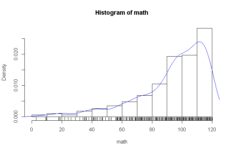
# 看看数学成绩的分布图

hist(math)

默认是按频数形成的直方图，设置freq参数可以画密度分布图。

hist(math, freq=FALSE)

lines(density(math), col='blue')

rug(jitter(math)) #轴须图，在轴旁边出现一些小线段，jitter是加噪函数

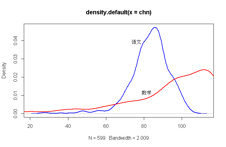
# 核密度图

plot(density(chn), col='blue', lwd=2)

lines(density(math), col='red', lwd=2)

text(locator(2),c("语文", "数学")) #用鼠标拾取点，加上文本标注

# 箱线图

boxplot(math)

boxplot.stats(math) #这个函数可以看到画出箱线图的具体的数据值

[1] 44 84 100 111 120

$n
[1] 599 #有效样本点个数

$conf
[1] 98.25696 101.74304

$out #离群值
[1] 38 42 35 40 43 36 41 40 36 18 26 36 42 32 41 29 18 24 10 20 34 19 10 3
[25] 35 20 35 18 22 9

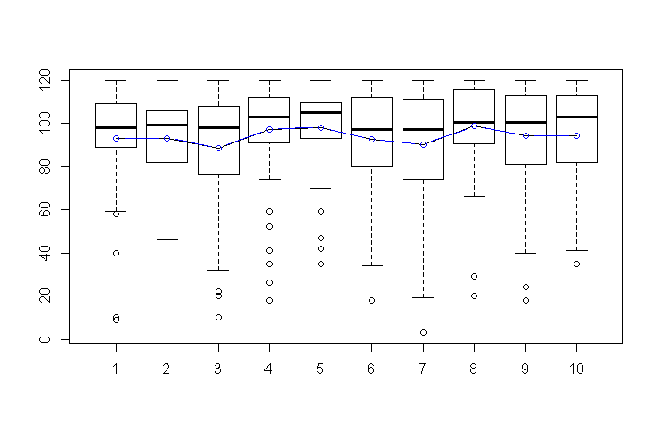
# 并列箱线图，看各班的数据分布情况

boxplot(math ~ class, data=scores)

lines(tapply(math,class,mean), col='blue', type='b') #加上平均值

可以看出2班没有拖后腿的，4班有6个拖后腿的

# 看看各科成绩的相关性

# 可以看出：数学和物理的相关性达88%，物理和化学成绩的相关性达86%。

cor(scores[,subjects])

               chn      math       eng       phy      chem politics       bio   history       geo        pe
chn      1.0000000 0.6588126 0.7326778 0.6578172 0.6271155 0.7257003 0.6902282 0.6971145 0.6438662 0.2712453
math     0.6588126 1.0000000 0.8079255 0.8860467 0.8304643 0.7090681 0.7951987 0.7732791 0.7723853 0.3300249
eng      0.7326778 0.8079255 1.0000000 0.8170998 0.7868710 0.7498946 0.7731044 0.7948219 0.7265406 0.3159347
phy      0.6578172 0.8860467 0.8170998 1.0000000 0.8615512 0.7081717 0.8077105 0.8100599 0.7814152 0.3251233
chem     0.6271155 0.8304643 0.7868710 0.8615512 1.0000000 0.6441334 0.7578770 0.7993298 0.7264814 0.2769066
politics 0.7257003 0.7090681 0.7498946 0.7081717 0.6441334 1.0000000 0.7071181 0.7192860 0.6906930 0.3033607
bio      0.6902282 0.7951987 0.7731044 0.8077105 0.7578770 0.7071181 1.0000000 0.7771735 0.8382525 0.2428081
history 0.6971145 0.7732791 0.7948219 0.8100599 0.7993298 0.7192860 0.7771735 1.0000000 0.7731044 0.2708434
geo      0.6438662 0.7723853 0.7265406 0.7814152 0.7264814 0.6906930 0.8382525 0.7731044 1.0000000 0.2605251
pe       0.2712453 0.3300249 0.3159347 0.3251233 0.2769066 0.3033607 0.2428081 0.2708434 0.2605251 1.0000000