第十八节,TensorFlow中使用批量归一化(BN)
在深度学习章节里,已经介绍了批量归一化的概念,详情请点击这里:第九节,改善深层神经网络:超参数调试、正则化以优化(下)
神经网络在进行训练时,主要是用来学习数据的分布规律,如果数据的训练部分和测试部分分布不一样,那么网络的泛化能力会变得非常差.而且对于训练的数据,每批分布也是不一样的,那么网络在迭代的过程中也要学习和适应不同的分布.这会大大降低网络的训练速度.此外,数据的分布对于激活函数来说也非常重要,有时数据分布范围太大不利于利用激活函数的非线性特性,比如激活函使用Sigmoid函数时,会导致训练时出现饱和的问题。而批量归一化就是为了缓解这个问题提出的。在实际应用中,批量归一化的收敛非常快,并且具有很强的泛化能力,某种情况下完全可以替代正则化和弃权。
一 批量归一化函数
归一化算法可以描述为:

其中xi是batch_size样本中的第i个样本,μB是求得的每个特征均值,σB2是求得每个特征的方差。
1.TensorFlow中自带BN函数的定义:
def batch_normalization(x,
                        mean,
                        variance,
                        offset,
                        scale,
                        variance_epsilon,
                        name=None):
各个参数的说明如下:
- x:代表任意维度的输入张量。
- mean:代表样本的均值。
- variance:代表样本的方差。
- offset:代表偏移,即相加一个转化值,也是公式中的beta。
- scale:代表缩放,即乘以一个转化值,也是公式中的gamma。
- variance_epsilon:是为了避免分母为0的情况下,给分母加上的一个极小值,默认即可。
- name:名称。
要想使用这个整数,必须由另一个函数配合使用,tf.nn.moments,由它来计算均值和方差,然后就可以使用BN了。
2.tf.nn.moment()函数的定义如下:
def moments(x, axes, shift=None, name=None, keep_dims=False):
- x:输入张量。
- axes:指定沿哪个轴计算平均值和方差。
- shift:A `Tensor` containing the value by which to shift the data for numerical stability, or `None` in which case the true mean of the data is used as shift. A shift close to the true mean provides the most numerically stable results.
- name:名称。
- keep_dims:是否保留维度,即形状是否和输入一样。
有了以上两个函数还不够,因为如果使用tf.nn.moment()函数计算均值和方差,我们需要保存每批次训练的均值和方差,然后求平均。为了有更好的效果,我们通常使用指数加权平均的方法来优化每次的均值和方差,于是就用到了tf.train.ExponentialMovingAverage()类,它的作用是让上一次的值对本次的值有个衰减后的影响,从而使每次的值连起来后会相对平滑一下:详细内容可以点击这里:第八节,改善深层神经网络:超参数调试、正则化以优化(中)
我们可以用一个表达式来表示这个函数的功能:
shadow_variable = decay * shadow_variable + (1 - decay) *variable
各参数说明如下:
- decay:代表衰减指数,是在ExponentialMovingAverage()中指定的,一般为0.9.
- variable:代表本批次样本中的值。
- 等式右边的shadow_variable:代表上次总样本的值。
- 等式左边的shadow_variable:代表本次次总样本的值。
对于shadow_variable的理解,你可以将其人为该数值表示的是1/(1-β)次的平均值,本次样本所占的权重为(1-decay),上次样本所占权重为(1-decay)decay,上上次样本所占权重为(1-decay)decay^2,以此类推....
3.tf.train.ExponentialMovingAverage类的定义如下:
  def __init__(self, decay, num_updates=None, zero_debias=False,
               name="ExponentialMovingAverage"):
 def apply(self, var_list=None):
参数说明如下:
- decay: Float. The decay to use.
- num_updates: Optional count of number of updates applied to variables. actual decay rate used is: `min(decay, (1 + num_updates) / (10 + num_updates))
- zero_debias: If `True`, zero debias moving-averages that are initialized with tensors.
- name: String. Optional prefix name to use for the name of ops added in.
-
var_list: A list of Variable or Tensor objects. The variables and Tensors must be of types float16, float32, or float64.apply
通过调用apply()函数可以更新指数加权平均值。
二 批量归一化的简单用法
上面的函数虽然参数不多,但是需要几个函数联合起来使用,于是TensorFlow中的layers模块里又实现了一次BN函数,相当于把几个函数合并到了一起,使用起来更加简单。下面来介绍一下,使用时需要引入:
from tensorflow.contrib.layers.python.layers import batch_norm
或者直接调用tf.contrib.layers.batch_norm(),该函数的定义如下:
def batch_norm(inputs,
               decay=0.999,
               center=True,
               scale=False,
               epsilon=0.001,
               activation_fn=None,
               param_initializers=None,
               param_regularizers=None,
               updates_collections=ops.GraphKeys.UPDATE_OPS,
               is_training=True,
               reuse=None,
               variables_collections=None,
               outputs_collections=None,
               trainable=True,
               batch_weights=None,
               fused=False,
               data_format=DATA_FORMAT_NHWC,
               zero_debias_moving_mean=False,
               scope=None,
               renorm=False,
               renorm_clipping=None,
               renorm_decay=0.99):
参数说明如下:
- inputs: A tensor with 2 or more dimensions, where the first dimension has `batch_size`. The normalization is over all but the last dimension if `data_format` is `NHWC` and the second dimension if `data_format` is `NCHW`.代表输入,第一个维度为batch_size
- dacay:Decay for the moving average. Reasonable values for `decay` are close to 1.0, typically in the multiple-nines range: 0.999, 0.99, 0.9, etc. Lower `decay` value (recommend trying `decay`=0.9) if model experiences reasonably good training performance but poor validation and/or test performance. Try zero_debias_moving_mean=True for improved stability.代表加权指数平均值的衰减速度,是使用了一种叫做加权指数衰减的方法更新均值和方差。一般会设置为0.9,值太小会导致均值和方差更新太快,而值太大又会导致几乎没有衰减,容易出现过拟合,这种情况一般需要把值调小点。
- center: If True, add offset of `beta` to normalized tensor. If False, `beta` is ignored. 指定是否使用偏移beta。
- scale: If True, multiply by `gamma`. If False, `gamma` is not used. When the next layer is linear (also e.g. `nn.relu`), this can be disabled since the scaling can be done by the next layer.是否进行变换(通过乘以一个gamma进行缩放),我们习惯在BN后面接一个线性变化,如Relu,所以scale一般都设置为Flase,因为后面有对数据的转换处理,所以这里就不用再处理了。
- epsilon: Small float added to variance to avoid dividing by zero.是为了避免分母为0的情况下,给分母加上的一个极小值,默认即可。
- activation_fn: Activation function, default set to None to skip it and maintain a linear activation.激活函数,默认为None,即使用线性激活函数。
- param_initializers: Optional initializers for beta, gamma, moving mean and moving variance.可选的初始化参数。
- param_regularizers: Optional regularizer for beta and gamma.可选的正则化项。
- updates_collections: Collections to collect the update ops for computation. The updates_ops need to be executed with the train_op. If None, a control dependency would be added to make sure the updates are computed in place.其变量默认是tf.GraphKeys.UPDATE_OPS,在训练时提供了一种内置的均值和方差更新机制,即通过图中的tf.Graphs.UPDATE_OPS变量来更新,但它是在每次当前批次训练完成后才更新均值和方差,这样就导致当前数据总是使用前一次的均值和方差,没有得到最新的更新。所以一般都会将其设置为None,让均值和方差即时更新。这样虽然相比默认值在性能上稍慢点,但是对模型的训练还是有很大帮助的。
- is_training: Whether or not the layer is in training mode. In training mode it would accumulate the statistics of the moments into `moving_mean` and `moving_variance` using an exponential moving average with the given `decay`. When it is not in training mode then it would use the values of the `moving_mean` and the `moving_variance`.当它为True,代表是训练过程,这时会不断更新样本集的均值与方差。当测试时,要设置成False,这样就会使用训练样本集的均值和方差。
- reuse: Whether or not the layer and its variables should be reused. To be able to reuse the layer scope must be given.支持共享变量,与下面的scope参数联合使用。
- variables_collections: Optional collections for the variables.
- outputs_collections: Collections to add the outputs.
- trainable: If `True` also add variables to the graph collection `GraphKeys.TRAINABLE_VARIABLES` (see `tf.Variable`).
- batch_weights: An optional tensor of shape `[batch_size]`, containing a frequency weight for each batch item. If present, then the batch normalization uses weighted mean and variance. (This can be used to correct for bias in training example selection.)
- used: Use nn.fused_batch_norm if True, nn.batch_normalization otherwise.
- data_format: A string. `NHWC` (default) and `NCHW` are supported.
- zero_debias_moving_mean: Use zero_debias for moving_mean. It creates a new air of variables 'moving_mean/biased' and 'moving_mean/local_step'.
- scope: Optional scope for `variable_scope`.指定变量的作用域variable_scope。
- renorm: Whether to use Batch Renormalization https://arxiv.org/abs/1702.03275). This adds extra variables during raining. The inference is the same for either value of this parameter.
- renorm_clipping: A dictionary that may map keys 'rmax', 'rmin', 'dmax' to scalar `Tensors` used to clip the renorm correction. The correction `(r, d)` is used as `corrected_value = normalized_value * r + d`, with `r` clipped to [rmin, rmax], and `d` to [-dmax, dmax]. Missing rmax, rmin, dmax are set to inf, 0, inf, respectively.
- renorm_decay: Momentum used to update the moving means and standard deviations with renorm. Unlike `momentum`, this affects training and should be neither too small (which would add noise) nor too large (which would give stale estimates). Note that `decay` is still applied to get the means and variances for inference.
三 为CIFAR10分类添加BN
这里继续在第十三节cifar10分类的代码基础上修改:
1.添加BN函数
def avg_pool_6x6(x):
    '''
    全局平均池化层,使用一个与原有输入同样尺寸的filter进行池化,'SAME'填充方式  池化层后
         out_height = in_hight / strides_height(向上取整)
         out_width = in_width / strides_width(向上取整)

    args;
        x:输入图像 形状为[batch,in_height,in_width,in_channels]
    '''
    return tf.nn.avg_pool(x,ksize=[1,6,6,1],strides=[1,6,6,1],padding='SAME')


def batch_norm_layer(value,is_training=False,name='batch_norm'):
    '''
    批量归一化  返回批量归一化的结果

    args:
        value:代表输入,第一个维度为batch_size
        is_training:当它为True,代表是训练过程,这时会不断更新样本集的均值与方差。当测试时,要设置成False,这样就会使用训练样本集的均值和方差。
              默认测试模式
        name:名称。
    '''
    if is_training is True:
        #训练模式 使用指数加权函数不断更新均值和方差
        return tf.contrib.layers.batch_norm(inputs=value,decay=0.9,updates_collections=None,is_training = True)
    else:
        #测试模式 不更新均值和方差,直接使用
        return tf.contrib.layers.batch_norm(inputs=value,decay=0.9,updates_collections=None,is_training = False)
2.为BN函数添加占位符参数
由于BN函数里需要设置是否为训练状态,所以需要定义一个占位符来传入我们处于训练模式还是测试模式。
#定义占位符
input_x = tf.placeholder(dtype=tf.float32,shape=[None,24,24,3])   #图像大小24x24x
input_y = tf.placeholder(dtype=tf.float32,shape=[None,10])        #0-9类别
is_training = tf.placeholder(dtype=tf.bool)                       #设置为True,表示训练 Flase表示测试
3。修改网络结构添加BN层
在第一层h_conv1和第二层h_conv2激活函数前添加BN层。
x_image = tf.reshape(input_x,[batch_size,24,24,3])

#1.卷积层 ->池化层 在激活函数之前追加BN层
W_conv1 = weight_variable([5,5,3,64])
b_conv1 = bias_variable([64])


h_conv1 = tf.nn.relu(batch_norm_layer(conv2d(x_image,W_conv1) + b_conv1,is_training=is_training))     #输出为[-1,24,24,64]
print_op_shape(h_conv1)
h_pool1 = max_pool_2x2(h_conv1)                                                                       #输出为[-1,12,12,64]
print_op_shape(h_pool1)


#2.卷积层 ->池化层   在激活函数之前追加BN层
W_conv2 = weight_variable([5,5,64,64])
b_conv2 = bias_variable([64])


h_conv2 = tf.nn.relu(batch_norm_layer(conv2d(h_pool1,W_conv2) + b_conv2,is_training=is_training))    #输出为[-1,12,12,64]
print_op_shape(h_conv2)
h_pool2 = max_pool_2x2(h_conv2)                                              #输出为[-1,6,6,64]
print_op_shape(h_pool2)


#3.卷积层 ->全局平均池化层
W_conv3 = weight_variable([5,5,64,10])
b_conv3 = bias_variable([10])

h_conv3 = tf.nn.relu(conv2d(h_pool2,W_conv3) + b_conv3)   #输出为[-1,6,6,10]
print_op_shape(h_conv3)

nt_hpool3 = avg_pool_6x6(h_conv3)                         #输出为[-1,1,1,10]
print_op_shape(nt_hpool3)
nt_hpool3_flat = tf.reshape(nt_hpool3,[-1,10])

y_conv = tf.nn.softmax(nt_hpool3_flat)
4 加入退化学习率
将原来的学习率改为退化学习率,让其每1000步衰退0.9.
#softmax交叉熵代价函数
cost = tf.reduce_mean(-tf.reduce_sum(input_y * tf.log(y_conv),axis=1))

#加入退化学习率 初始值为learning_rate,让其每1000步,衰减0.9  学习率 = learning_rate*0.9^(global_step/1000)
global_step = tf.Variable(0,trainable=False)
decaylearning_rate = tf.train.exponential_decay(learning_rate,global_step,1000,0.9)

#求解器    执行一次train global_step变量会自加1
train = tf.train.AdamOptimizer(learning_rate).minimize(cost,global_step = global_step)

#返回一个准确度的数据
correct_prediction = tf.equal(tf.arg_max(y_conv,1),tf.arg_max(input_y,1))
#准确率
accuracy = tf.reduce_mean(tf.cast(correct_prediction,dtype=tf.float32))
5 开始训练
这这里我们需要给BN函数传入一个is_training参数,表明当前是在训练模式还是处于测试模式。
'''
四 开始训练
'''
sess = tf.Session();
sess.run(tf.global_variables_initializer())
# 启动计算图中所有的队列线程 调用tf.train.start_queue_runners来将文件名填充到队列,否则read操作会被阻塞到文件名队列中有值为止。
tf.train.start_queue_runners(sess=sess)

for step in range(training_step):
    #获取batch_size大小数据集
    image_batch,label_batch = sess.run([images_train,labels_train])

    #one hot编码
    label_b = np.eye(10,dtype=np.float32)[label_batch]

    #开始训练      执行一次train global_step变量会自加1,这样decaylearning_rate值就会改变
    rate,_ = sess.run([decaylearning_rate,train],feed_dict={input_x:image_batch,input_y:label_b,is_training:True})

    if step % display_step == 0:
        train_accuracy = sess.run(accuracy,feed_dict={input_x:image_batch,input_y:label_b,is_training:False})
        print('Step {0} tranining accuracy {1}'.format(step,train_accuracy))

image_batch, label_batch = sess.run([images_test, labels_test])
label_b = np.eye(10,dtype=np.float32)[label_batch]
test_accuracy = sess.run(accuracy,feed_dict={input_x:image_batch,input_y:label_b,is_training:False})
print('finished! test accuracy {0}'.format(test_accuracy))

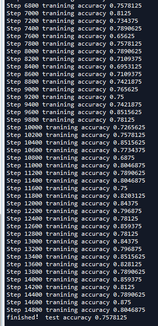
可以看到准确率有了很大的提升,比第十三节的70%提升了很多,训练时的准确率已经达到了80%左右,然而测试时模型的准确率下降了不少。除此之外,我们可以使用cifar10_input中的distorted_inputs()函数来增大数据集,或者采用一些过拟合的方法继续优化。

 浙公网安备 33010602011771号