

算法初探:Tensorflow及PAI平台的使用
前言
Tensorflow这个词由来已久,但是对它的理解一直就停留在“听过”的层面。之前做过一个无线图片适配问题智能识别的项目,基于Tensorflow实现了GoogLeNet - Inception V3网络(一种包含22层的深层卷积神经网络),但是基本上也属于“盲人摸象”、“照葫芦画瓢”的程度。作为当今机器学习乃至深度学习界出现频率最高的一个词,有必要去了解一下它到底是个什么东西。
而PAI,作为一站式地机器学习和算法服务平台,它大大简化了模型构建、模型训练、调参、模型性能评估、服务化等一系列算法的工作,可以帮助我们更快捷地实现算法实验和应用。
一、Tensorflow初探
1. 安装和启动
因为我自己的mac-pro安装了docker,所以安装Tensorflow的环境非常简单,只要拉取Tensorflow的官方镜像就可以完成Tensorflow的环境搭建。
#拉取tensorflow镜像
docker pull tensorflow/tensorflow

#创建一个tensorflow的工作目录,挂载到容器内
mkdir -p /Users/znifeng/docker-data/tensorflow/notebooks

#启动容器
docker run -it --rm --name myts -v /Users/znifeng/docker-data/tensorflow/notebooks:/notebooks -p 8888:8888 tensorflow/tensorflow
启动成功后,将看到如下信息: 

复制链接http://127.0.0.1:8888/?token=487c52e0aa0cd2a7b231bf909c1d6666482f8ed03353e510到浏览器,就可以看到jupyter(支持在线编写和调试python的交互式笔记本)页面:
 
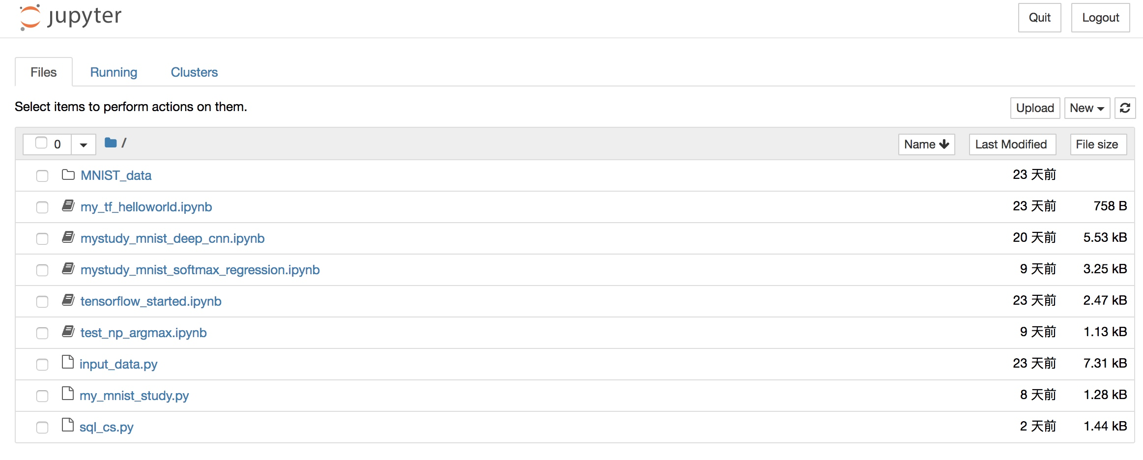
接下来,你可以在jupyter上或者在docker容器内部编写和调试tensorflow的代码,容器内部已经包含了tensorflow的所有库。
2. 基本使用
2.1 核心概念
- 使用图(graph)来表示计算任务
- 使用张量(tensor)来表示数据。张量与矢量的区别:矢量相当于一阶的张量,张量可以从0阶到多阶(多维)
- 图中的每一个节点称之为op(operation),每一个op有0或多个Tensor作为输入,执行计算后产出0或多个Tensor作为输出
- 在被称之为会话Session的上下文(context)中执行图
- 通过变量(variable)来维护状态
- 使用feed和fetch可以为任意的操作赋值或者从其中获取数据
- 使用placeholder来定义占位符,在运行时传入对应的参数值
TensorFlow程序通常被组织成一个构建阶段和一个执行阶段。在构建阶段,op的执行步骤被描述成一个图,在执行阶段,使用会话执行图中的op。在Python中,返回的tensor是numpy.ndarray对象。;在C/C++中,返回的是tensorflow:Tensor实例。
2.2 使用示例
2.2.1 第一个helloworld程序:
import tensorflow as tf

#第一阶段: 构建图
#定义一个1x2的矩阵,矩阵元素为[3 3]
matrix1 = tf.constant([[3., 3.]])

#定义一个2x1的矩阵,矩阵元素为[2
                           2]
matrix2 = tf.constant([[2.],[2.]])

# 创建一个矩阵乘法 matmul op , 把 'matrix1' 和 'matrix2' 作为输入.
product = tf.matmul(matrix1, matrix2)

#第二阶段: 执行图
with tf.Session() as sess:
    print "matrix1: %s" % sess.run(matrix1)
    print "matrix2: %s" % sess.run(matrix2)
    print "result type: %s" % type(sess.run(product))
    print "result: %s" % sess.run(product)
输出结果:
matrix1: [[3. 3.]]
matrix2: [[2.]
 [2.]]
result type: <type 'numpy.ndarray'>
result: [[12.]]
如上图所示,在第一阶段(构建图)中,我们的每一行操作其实都是一个operation,包含两个constant操作和一个矩阵相乘的操作,每个operation的输出都是tensor,它的类型是num.ndarray。实际上,构建阶段我们只是定义op,并不会真正去执行;而在第二阶段中,通过定义了一个会话session,我们才会在会话中真正开始执行前面定义的各个operation,然后获得执行的结果。
2.2.2 使用tensorflow实现识别手写数字(1~9)模型 —— Softmax Regression
import input_data
mnist = input_data.read_data_sets("MNIST_data/", one_hot=True)

import tensorflow as tf

##Define input data format
#input images, each image is represented by a tensor of 784 dimensions
x = tf.placeholder("float", [None,784])
#input labels, each label values one digit of [0,9], which is represented by a tensor of 10 dimensions
y_ = tf.placeholder("float", [None, 10])

##Define Model and algorithm
#weight array of each feature VS predicted result
W = tf.Variable(tf.zeros([784, 10]))
#bias of each digit
b = tf.Variable(tf.zeros([10]))
#predicted probability array of an image, which is of 10 dimensions.
#tf.matmul:矩阵相乘
y = tf.nn.softmax(tf.matmul(x,W) + b)
#cross-entropy or called loss function
#tf.reduce_sum:压缩求和: tf.reduce_sum(x, 0)将x按行求和,tf.reduce_sum(x, 1)将x按列求和,tf.reduce_sum(x, [0, 1])按行列求和
cross_entropy = -tf.reduce_sum(y_*tf.log(y))
#gredient descent algorithm
train_step = tf.train.GradientDescentOptimizer(0.01).minimize(cross_entropy)

##Training model
#initialize all variables
init = tf.global_variables_initializer()
with tf.Session() as sess:
    sess.run(init)
    for i in range(1000):
        batch_xs, batch_ys = mnist.train.next_batch(100)
        sess.run(train_step, feed_dict={x: batch_xs, y_:batch_ys})

    ##Evaluation
    #tf.argmax(vector, 1):返回的是vector中的最大值的索引号。tf.argmax(vector, 0)
    correct_prediction = tf.equal(tf.argmax(y,1), tf.argmax(y_,1))
    accuracy = tf.reduce_mean(tf.cast(correct_prediction, "float"))
    print sess.run(accuracy, feed_dict={x: mnist.test.images, y_: mnist.test.labels})
输出结果:
0.904
模型中使用的数据来自tensorflow/g3doc/tutorials/mnist/,总共包含7万张784(28x28)像素的1~9的数字图片,其中55000张用于模型训练作为训练集,5000张作为验证集,剩余10000张用作测试集。
因此,每一张图片都可以用一个784维的向量来表示,向量里的每一个元素表示某个像素的强度值,介于0和1之间。使用x = tf.placeholder("float", [None,784])表示输入集x,其中placeholder为占位符,在实际使用时,我们再通过feed传入具体的行数来替换其中的None。y_则为对应的实际结果,因为结果集合为0~9,因此我们可以用[y0,y1,...,y9]的十维向量来表示结果,比如数字“1”可以表示为[0,1,0,0,0,0,0,0,0,0]。本例中,定义的模型为线性模型,先用wx+b得到初步结果z,再通过softmax函数将z折射得到0~9各个数字的概率值。
 

在模型求解时,我们需要定义一个指标来评估模型是好的。而在机器学习中,通常是定义指标来表示模型是坏的,然后尽量最小化该指标得到最优解,该指标也称为成本(cost)或损失(loss)函数。本例中,我们用“交叉熵”来作为损失函数cross_entropy = -tf.reduce_sum(y_*tf.log(y)),然后用梯度下降的方式求解train_step = tf.train.GradientDescentOptimizer(0.01).minimize(cross_entropy)。其中0.01为下降的速率。
可以看到,经过1000次迭代,我们的模型的预测结果的准确率达到了90.4%。
2.2.3 使用tensorflow实现识别手写数字(1~9)模型 —— DeepCNN
上节中用softmax模型预测的准确率大概在90%,接下来尝试下用tensorflow实现一个卷积神经网络模型来识别手写数字。
import input_data
mnist = input_data.read_data_sets("MNIST_data/", one_hot=True)

import tensorflow as tf
def weight_variable(shape):
    initial = tf.truncated_normal(shape, stddev=0.1)
    return tf.Variable(initial)

def bias_variable(shape):
    initial = tf.constant(0.1, shape=shape)
    return tf.Variable(initial)

def conv2d(x, W):
    return tf.nn.conv2d(x, W, strides=[1,1,1,1], padding="SAME")

def max_pool_2x2(x):
    return tf.nn.max_pool(x, ksize=[1, 2, 2, 1], strides=[1, 2, 2, 1], padding='SAME')

x = tf.placeholder("float", shape=[None, 784])
y_ = tf.placeholder("float", shape=(None, 10))

#第一层卷积
W_conv1 = weight_variable([5, 5, 1, 32])
b_conv1 = bias_variable([32])
x_image = tf.reshape(x, [-1,28,28,1])
h_conv1 = tf.nn.relu(conv2d(x_image, W_conv1) + b_conv1)
h_pool1 = max_pool_2x2(h_conv1)

#第二层卷积
W_conv2 = weight_variable([5, 5, 32, 64])
b_conv2 = bias_variable([64])
h_conv2 = tf.nn.relu(conv2d(h_pool1, W_conv2) + b_conv2)
h_pool2 = max_pool_2x2(h_conv2)

#密集连接层
W_fc1 = weight_variable([7 * 7 * 64, 1024])
b_fc1 = bias_variable([1024])
h_pool2_flat = tf.reshape(h_pool2, [-1, 7*7*64])
h_fc1 = tf.nn.relu(tf.matmul(h_pool2_flat, W_fc1) + b_fc1)

#Dropout防止过拟合
keep_prob = tf.placeholder("float")
h_fc1_drop = tf.nn.dropout(h_fc1, keep_prob)

#输出层: softmax
W_fc2 = weight_variable([1024, 10])
b_fc2 = bias_variable([10])
y_conv=tf.nn.softmax(tf.matmul(h_fc1_drop, W_fc2) + b_fc2)

#训练和评估模型
cross_entropy = -tf.reduce_sum(y_*tf.log(y_conv))
train_step = tf.train.AdamOptimizer(1e-4).minimize(cross_entropy)
correct_prediction = tf.equal(tf.argmax(y_conv,1), tf.argmax(y_,1))
accuracy = tf.reduce_mean(tf.cast(correct_prediction, "float"))

with tf.Session() as sess:
    sess.run(tf.global_variables_initializer())
    for i in range(2000):
        batch = mnist.train.next_batch(50)
        if i%200 == 0:
            train_accuracy = sess.run(accuracy, feed_dict={x:batch[0], y_: batch[1], keep_prob: 1.0})
            print "step %d, training accuracy %g"%(i, train_accuracy)
        train_step.run(feed_dict={x: batch[0], y_: batch[1], keep_prob: 0.5})
    print "final training accuracy %g" % sess.run(accuracy, feed_dict={x:batch[0], y_: batch[1], keep_prob: 1.0})
输出结果:
step 0, training accuracy 0.14
step 200, training accuracy 0.92
step 400, training accuracy 0.96
step 600, training accuracy 1
step 800, training accuracy 0.9
step 1000, training accuracy 0.96
step 1200, training accuracy 0.94
step 1400, training accuracy 0.94
step 1600, training accuracy 0.98
step 1800, training accuracy 1
final training accuracy 0.99
可以看到,2000次迭代后,deepccn的预测准确率达到了:99%。
二、PAI平台的使用
前面介绍了Tensorflow的基本概念和使用,下面简单介绍下使用PAI完成LR模型训练的基本过程。整个流程大概包含以下步骤:离线数据开发 -> PAI平台实验搭建 -> 模型服务化
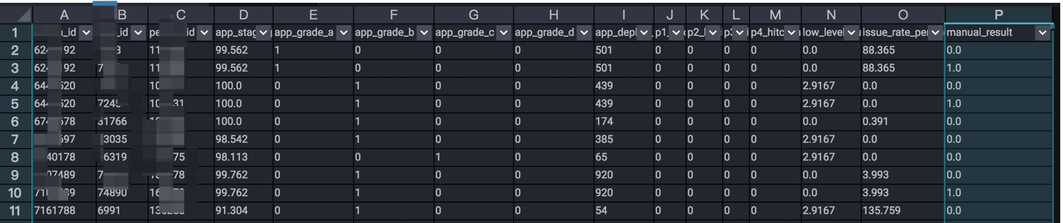
2.1 离线数据开发
首先,算法的基础是数据,我们首先要通过对业务的分析,找出影响目标结果的特征,并对特征数据进行采集,得到各项特征的原始数据。这一部分,可以在odps完成。如“需求风险智能识别”中,涉及到多个表的join和指标的提取、计算等,对于一些缺省的值可以按照不同的策略来填充(如用0填充,或者该项的平均值)。最终得到如下的训练数据:
 
2.2 PAI平台实验搭建
进入PAI平台中,新建实验:smarttest,搭建如下的实验流程:
 
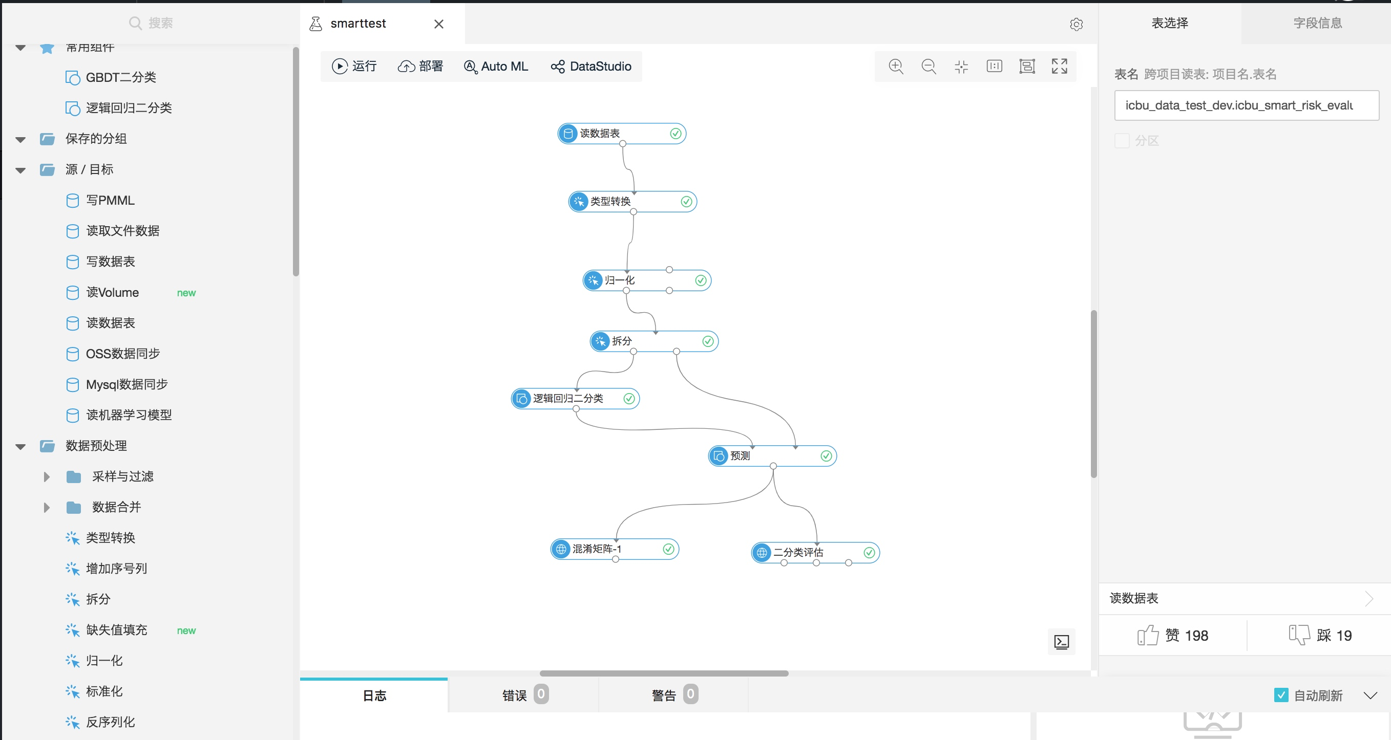
流程中的每个组件可以从左侧“组件”导航栏中获取。具体流程如下:
- 读数据表:输入odps表名
- 类型转换:将特定的字段统一转化为double/int类型
- 归一化:选取用于训练的特征,并进行归一化。归一化的逻辑为:
y= (x-MinValue)/(MaxValue-MinValue) - 拆分:将数据集按照比例拆分为训练集和测试集
- 逻辑回归二分类:使用LR模型对训练集的数据进行训练
- 预测:将训练得到的模型对测试集的输入数据进行预测
- 混淆矩阵:产出模型预测结果的混淆矩阵
- 二分类评估:得到模型评估的AUC、KS、F1 Score等结果
2.3 模型服务化
训练好模型后,就可以将模型在线服务化。


 浙公网安备 33010602011771号