Machine Learning - Classification Tree in Python

 Import Modules:

import numpy as np
import pandas as pd
import matplotlib.pyplot as plt

from sklearn.model_selection import train_test_split
from sklearn.model_selection import cross_val_score
from sklearn.tree import DecisionTreeClassifier  # to build a classification tree
from sklearn.tree import plot_tree  # to draw a classification tree
from sklearn.metrics import confusion_matrix  # to create a confusion matrix
# from sklearn.metrics import plot_confusion_matrix  # deprecated
from sklearn.metrics import ConfusionMatrixDisplay  # to draw a confusion matrix

 

Import Data:

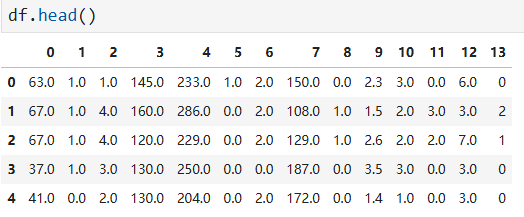
# df = pd.read_csv('heart+disease/processed.cleveland.data', header=None)

df = pd.read_csv('https://archive.ics.uci.edu/ml/machine-learning-databases/heart-disease/processed.cleveland.data', header=None)

 

 

Variables Table

Variable Name	Role	Type	Demographic	Description	Units	Missing Values
age	Feature	Integer	Age		years	no
sex	Feature	Categorical	Sex			no
cp	Feature	Categorical				no
trestbps	Feature	Integer		resting blood pressure (on admission to the hospital)	mm Hg	no
chol	Feature	Integer		serum cholestoral	mg/dl	no
fbs	Feature	Categorical		fasting blood sugar > 120 mg/dl		no
restecg	Feature	Categorical				no
thalach	Feature	Integer		maximum heart rate achieved		no
exang	Feature	Categorical		exercise induced angina		no
oldpeak	Feature	Integer		ST depression induced by exercise relative to rest		no
slope	Feature	Categorical				no
ca	Feature	Integer		number of major vessels (0-3) colored by flourosopy		yes
thal	Feature	Categorical				yes
num	Target	Integer		diagnosis of heart disease (the predicted attribute)		no

 

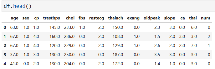
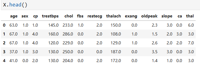
# change the column numbers to column names
df.columns = [
    'age',
    'sex',
    'cp',
    'trestbps',
    'chol',
    'fbs',
    'restecg',
    'thalach',
    'exang',
    'oldpeak',
    'slope',
    'ca',
    'thal',
    'num'
]

 

 

Missing Data Part 1: Identify Missing Data:

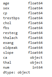
df.dtypes

 

 

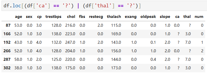
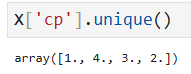
df['ca'].unique()
# array(['0.0', '3.0', '2.0', '1.0', '?'], dtype=object)

df['thal'].unique()
# array(['6.0', '3.0', '7.0', '?'], dtype=object)

len(df.loc[(df['ca'] == '?') | (df['thal'] == '?')])
# 6

 

 

Missing Data Part 2: Deal with Missing Data:

df_no_missing = df.loc[(df['ca'] != '?') & (df['thal'] != '?')]

len(df_no_missing)
# 297

 

Format the Data Part 1: Split the Data into Dependent and Independent Variables

# Make a new copy of the columns used to make prediction
X = df_no_missing.drop('num', axis=1).copy()  # alternatively: X = df_no_missing.iloc[:, :-1]

 

 

# Make a new copy of the column we want to predict
y = df_no_missing['num'].copy()

 

 

Format the Data Part 2: One-Hot Encoding

 

 

 

 

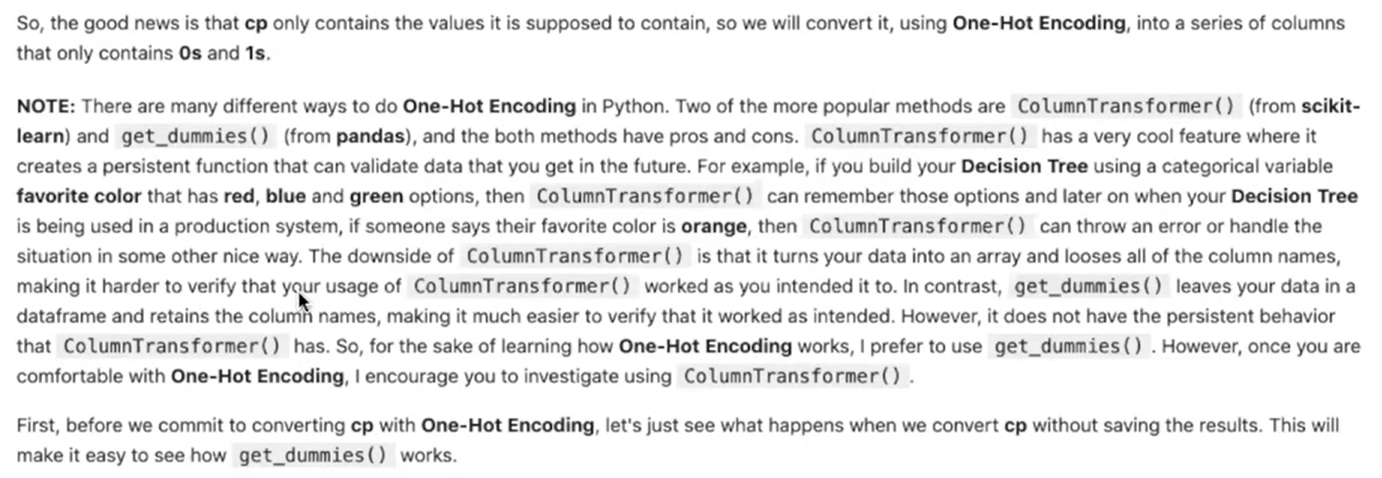
pd.get_dummies(X, columns=['cp']).head()

 

 

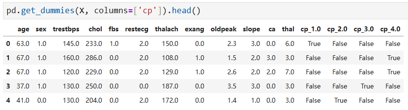
X_encoded = pd.get_dummies(X, columns=['cp',
                                       'restecg', 
                                       'slope', 
                                       'thal'])

 

pd.set_option('display.max_columns', None)
X_encoded.head()

 

 

 

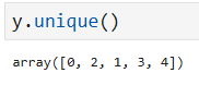
y_not_zero_index = y > 0
y[y_not_zero_index] = 1

y.unique()
# array([0, 1])

 

Build a Preliminary Classification Tree

X_train, X_test, y_train, y_test = train_test_split(X_encoded, y, random_state=42)

clf_dt = DecisionTreeClassifier(random_state=42)
clf_dt = clf_dt.fit(X_train, y_train)

 

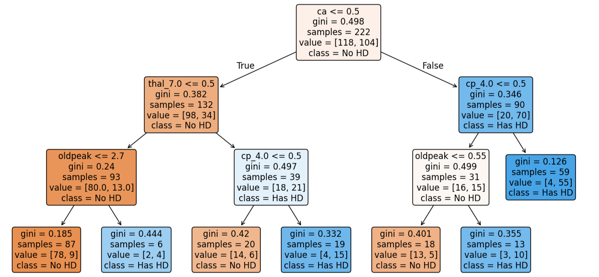
plt.figure(figsize=(15, 7.5))
plot_tree(clf_dt,
          filled=True,
          rounded=True,
          class_names=['No HD', 'Yes HD'],
          feature_names=X_encoded.columns)

 

 

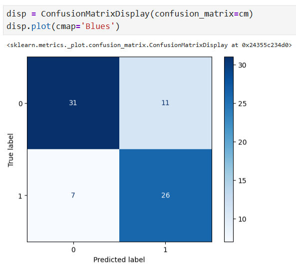
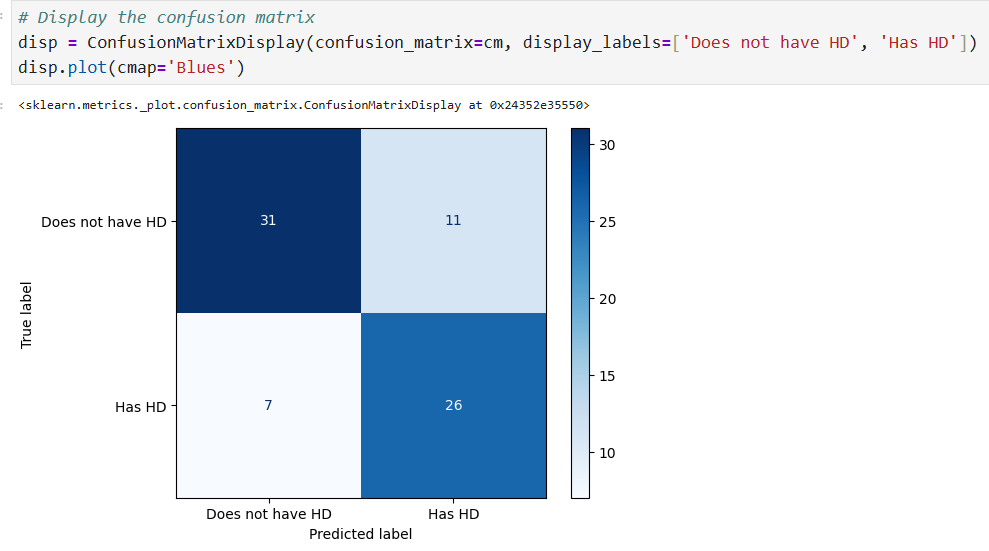
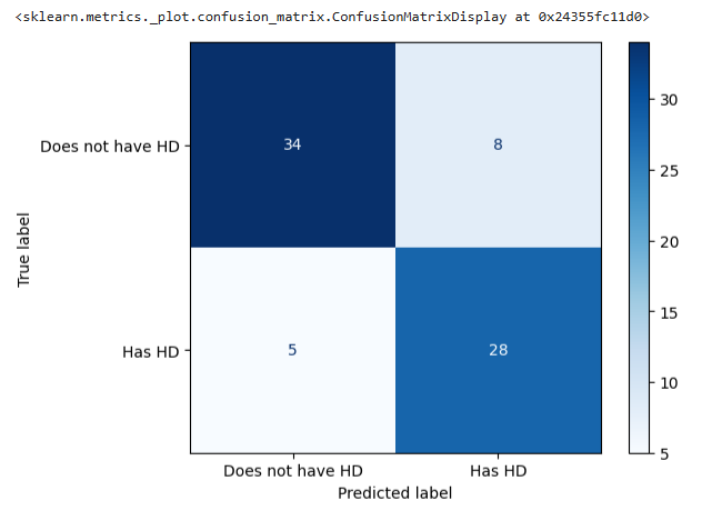
y_pred = clf_dt.predict(X_test)

# Compute confusion matrix
cm = confusion_matrix(y_test, y_pred)

# Display the confusion matrix
disp = ConfusionMatrixDisplay(confusion_matrix=cm, display_labels=['Does not have HD', 'Has HD'])
disp.plot(cmap='Blues')

 

          

 

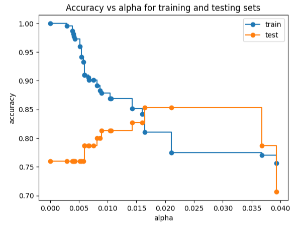
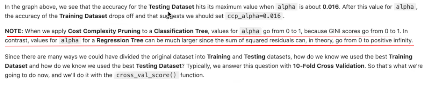
Cost Complexity Pruning Part 1: Visualize alpha

 

path = clf_dt.cost_complexity_pruning_path(X_train, y_train)  # determine values for alpha
ccp_alphas = path.ccp_alphas  # extract difference values for alpha
ccp_alphas = ccp_alphas[:-1]  # exclude the maximum value for alpha

clf_dts = []  # create an array that we will put decision tress into

# create one decision tree per value for alpha and store it in the array
for ccp_alpha in ccp_alphas:
    clf_dt = DecisionTreeClassifier(random_state=42, ccp_alpha=ccp_alpha)
    clf_dt.fit(X_train, y_train)
    clf_dts.append(clf_dt)

 

train_scores = [clf_dt.score(X_train, y_train) for clf_dt in clf_dts]
test_scores = [clf_dt.score(X_test, y_test) for clf_dt in clf_dts]

fig, ax = plt.subplots()
ax.set_xlabel('alpha')
ax.set_ylabel('accuracy')
ax.set_title('Accuracy vs alpha for training and testing sets')
ax.plot(ccp_alphas, train_scores, marker='o', label='train', drawstyle='steps-post')
ax.plot(ccp_alphas, test_scores, marker='o', label='test', drawstyle='steps-post')
ax.legend()
plt.show()

 

 

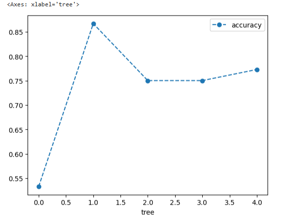
Cost Complexity Pruning Part 2: Cross Validation for Finding the Best Alpha

 

clf_dt = DecisionTreeClassifier(random_state=42, ccp_alpha=0.016)  # create the tree with alpha=0.016

# now use 5-fold cross validation create 5 different training and testing datasets that
# are then used to train and test the tree.
# NOTE: We use 5-fold because we don't have tons of data.
scores = cross_val_score(clf_dt, X_train, y_train, cv=5)
df = pd.DataFrame(data={'tree': range(5), 'accuracy': scores})

df.plot(x='tree', y='accuracy', marker='o', linestyle='--')

 

 

 

# create an array to store the results of each fold during cross validation
alpha_loop_values = []

# For each candidate value for alpha, we will ran 5-fold cross validation
# Then we will store the mean and standard deviation of the scores (the accuracy) for each call
# to cross_val_score in alpha_loop_values.
for ccp_alpha in ccp_alphas:
    clf_dt = DecisionTreeClassifier(random_state=42, ccp_alpha=ccp_alpha)
    scores = cross_val_score(clf_dt, X_train, y_train, cv=5)
    alpha_loop_values.append([ccp_alpha, np.mean(scores), np.std(scores)])

 

# Now we can draw a graph of the means and standard deviations of the scores 
# for each candidate value for alpha
alpha_results = pd.DataFrame(alpha_loop_values, columns=['alpha', 'accuracy_mean', 'accuracy_std'])

alpha_results.plot(x='alpha', 
                   y='accuracy_mean',
                   yerr='accuracy_std',
                   marker='o', 
                   linestyle='--')

 

 

 

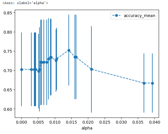
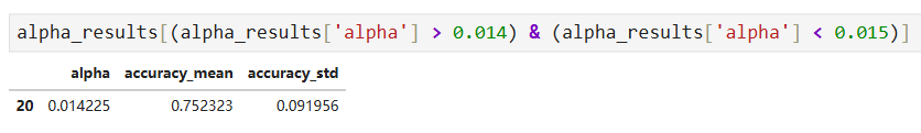
# Store the ideal value for alpha so that we can use it to build the best tree.
ideal_ccp_alpha = alpha_results[(alpha_results['alpha'] > 0.014) & (alpha_results['alpha'] < 0.015)]['alpha']

 

 

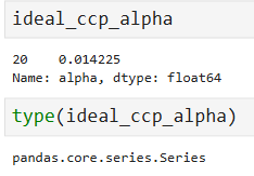
ideal_ccp_alpha = float(ideal_ccp_alpha.iloc[0])

ideal_ccp_alpha
# 0.014224751066856332

 

Build, Evaluate, Draw and Interpret the Final Classification Tree

# Draw another confusion matrix to see if the pruned tree does better.
y_pred = clf_dt_pruned.predict(X_test)
cm = confusion_matrix(y_test, y_pred)
disp = ConfusionMatrixDisplay(confusion_matrix=cm, display_labels=['Does not have HD', 'Has HD'])
disp.plot(cmap='Blues')

 

 

 

plt.figure(figsize=(15, 7.5))
plot_tree(clf_dt_pruned, 
          filled=True, 
          rounded=True, 
          class_names=['No HD', 'Has HD'], 
          feature_names=X_encoded.columns)