Machine Learning - Principal Component Analysis (PCA) Part I

 

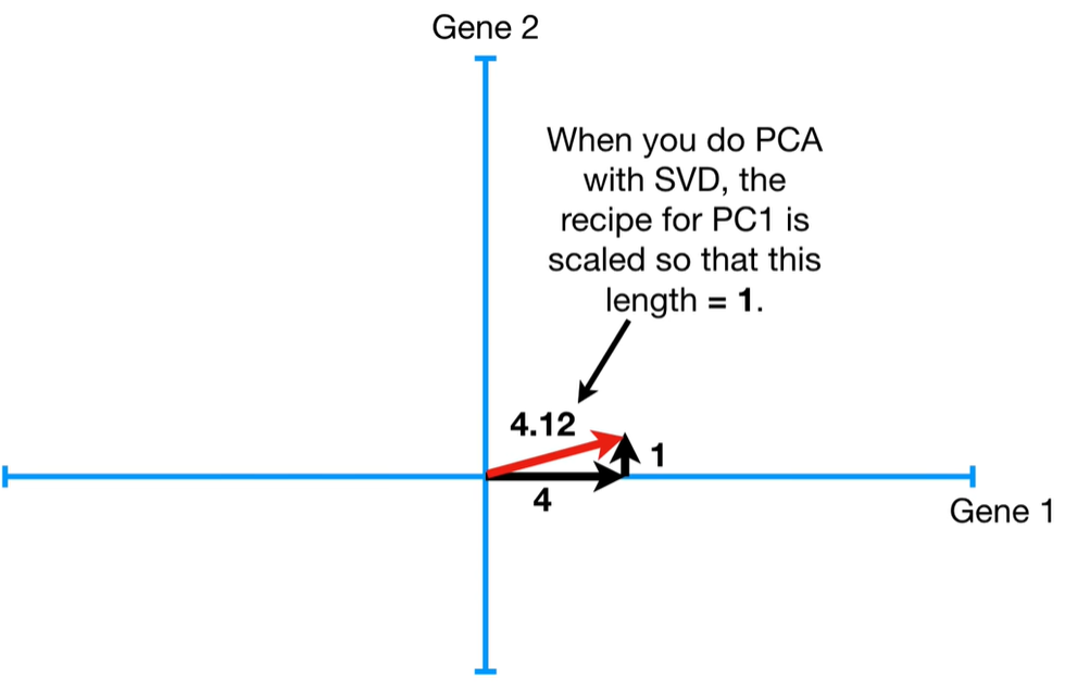
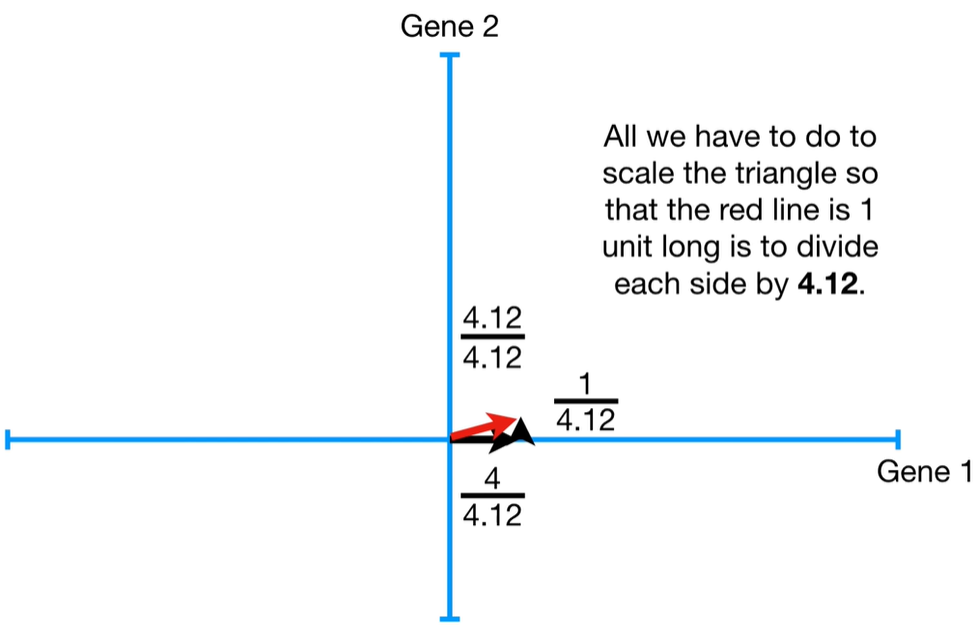
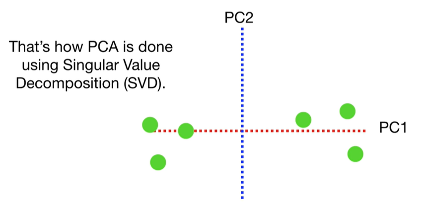
     SVD

 

 

 

 

 

 

 

 

 

 

 

 

 

 

 

     

 

 

 

 

 

 

 

     

 

     

 

     

 

 

 

 

 

 

 

 

 

 

 

 

 

 

 

 

 

 

 

 

 

 

     

 

 

     

 

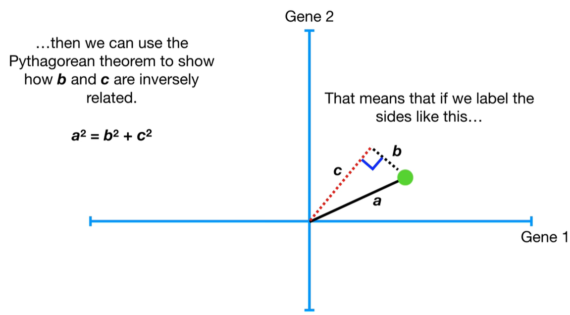
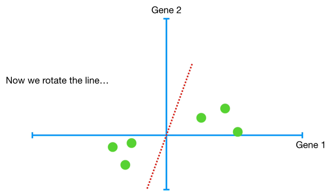
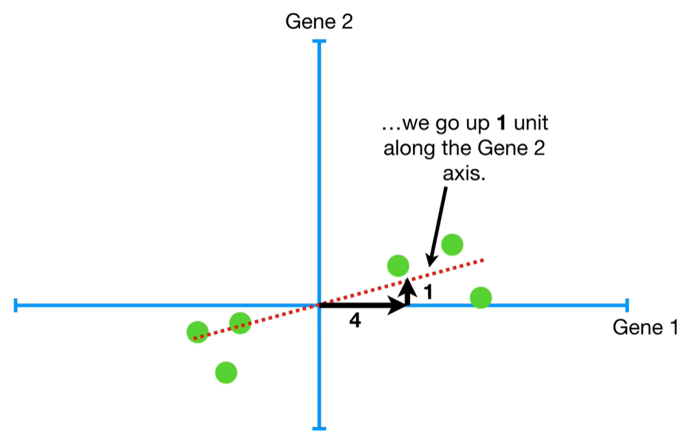
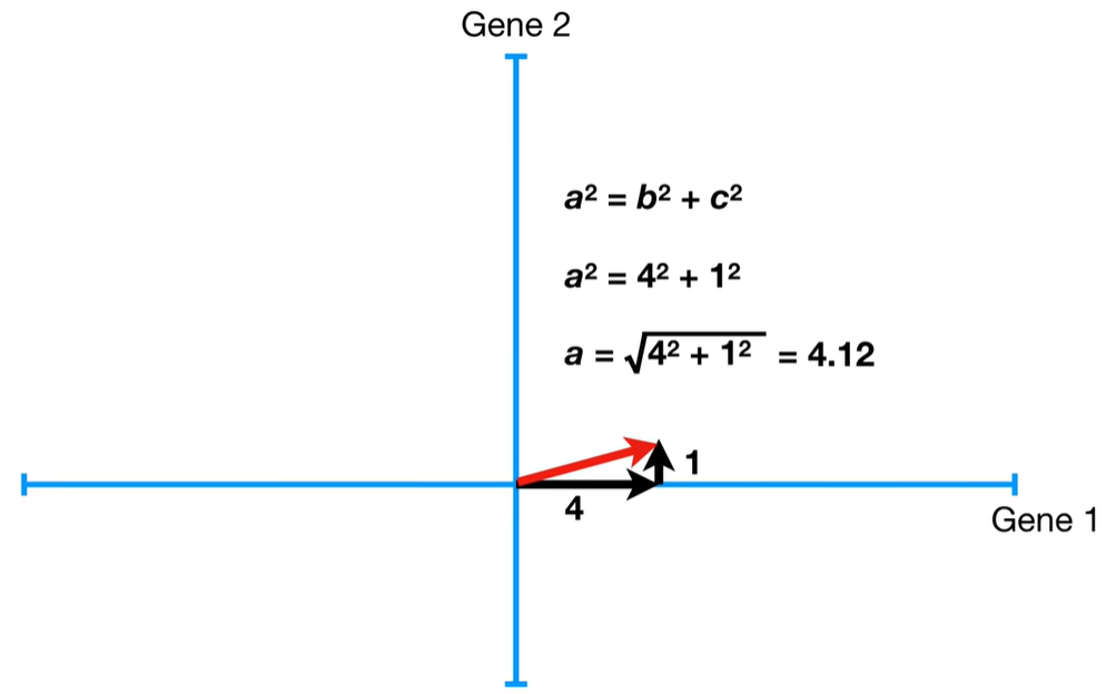
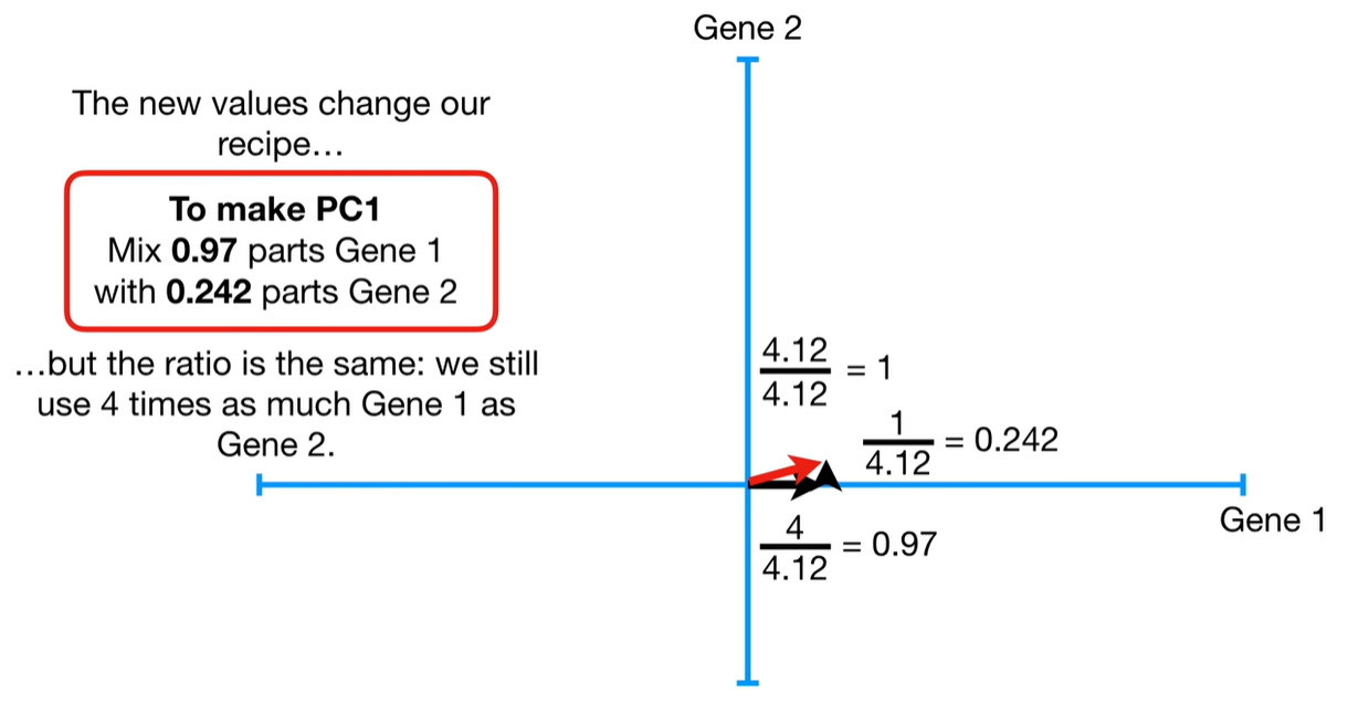
     understand the variables vectors rather than scalers

 

 

 

 

 

 

 

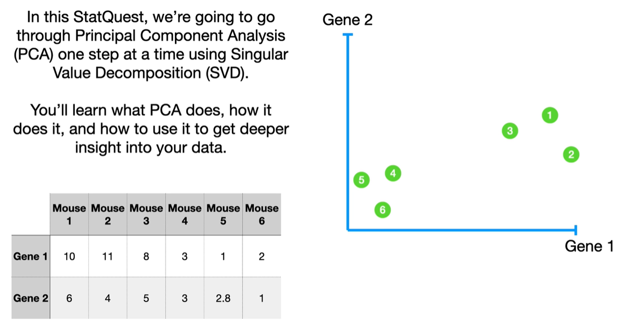
Step-by-step process to calculate eigenvalues in PCA

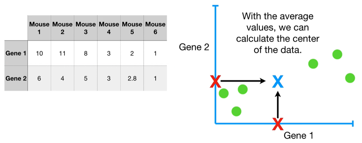
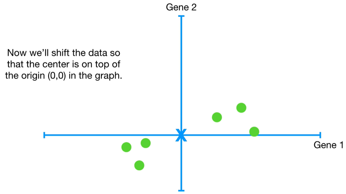
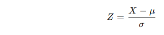
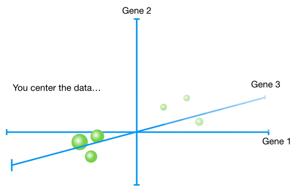
✅ Step 1: Standardize the data

Before applying PCA, standardize your data to have mean = 0 and standard deviation = 1 for each feature (unless already standardized).

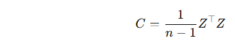
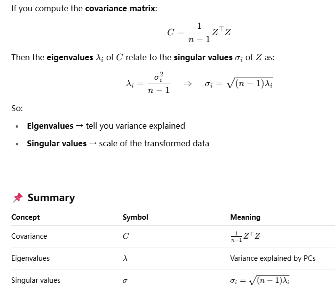
✅ Step 2: Compute the covariance matrix

Let the standardized data matrix be Z (with shape n×p, where n is the number of samples and p the number of features). The covariance matrix is:

C will be a p×p matrix.

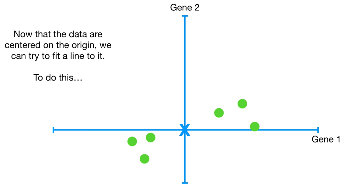
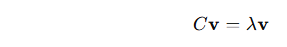
✅ Step 3: Compute eigenvalues and eigenvectors

You now solve the eigenvalue problem for the covariance matrix:

• λ are the eigenvalues (scalars)

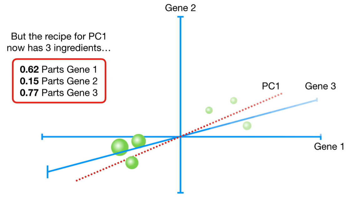
• v are the eigenvectors (principal components)

The eigenvalues are the solutions to the characteristic equation:

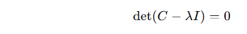
Use numerical methods (e.g. in Python with NumPy) to compute these.

💡 Interpretation

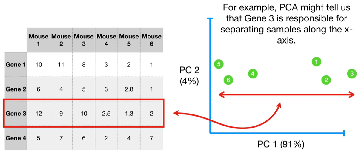
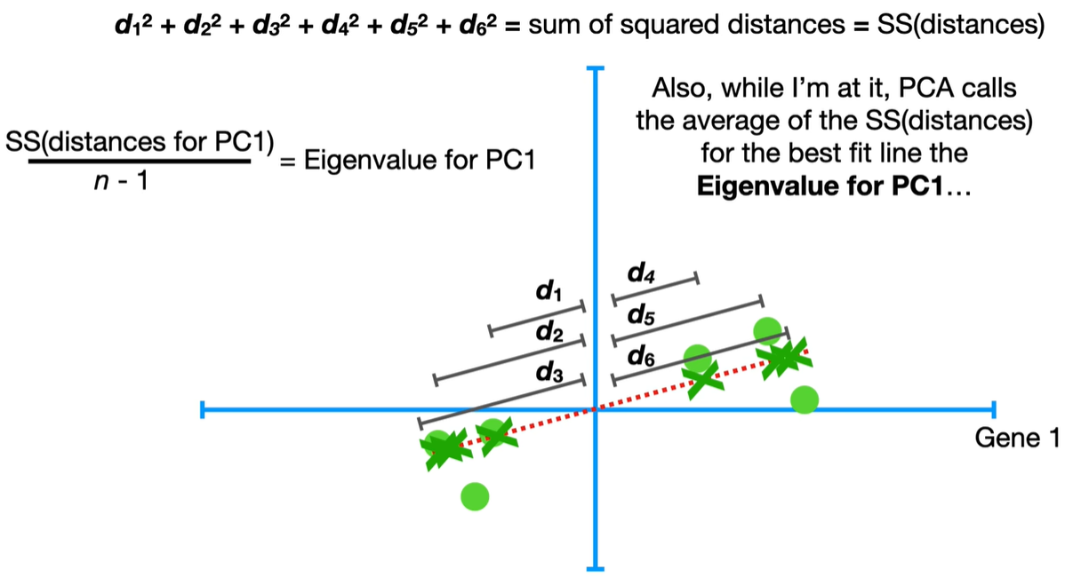
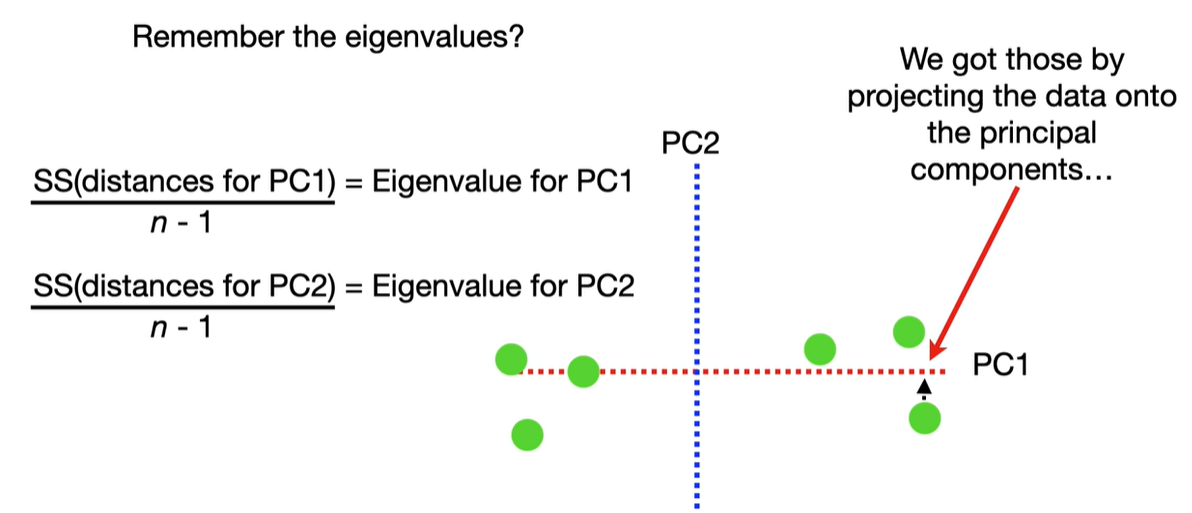
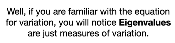
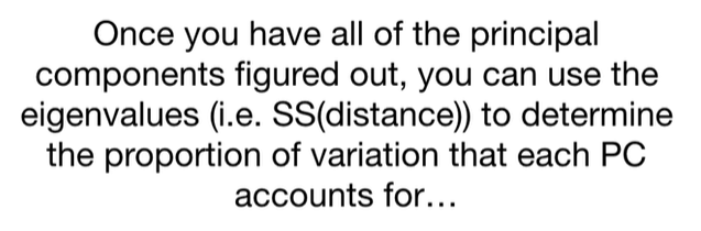
• Each eigenvalue λi​ indicates the variance explained by the corresponding principal component.

• The sum of all eigenvalues equals the total variance in the dataset.

• Larger eigenvalues → more important principal components.

 

import numpy as np

# Example data (rows = samples, columns = features)
X = np.array([[2.5, 2.4],
              [0.5, 0.7],
              [2.2, 2.9],
              [1.9, 2.2],
              [3.1, 3.0]])

# Step 1: Standardize the data
X_centered = X - np.mean(X, axis=0)

# Step 2: Covariance matrix
cov_matrix = np.cov(X_centered, rowvar=False)

# Step 3: Eigenvalues and eigenvectors
eigenvalues, eigenvectors = np.linalg.eig(cov_matrix)

print("Eigenvalues:", eigenvalues)

 

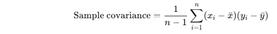
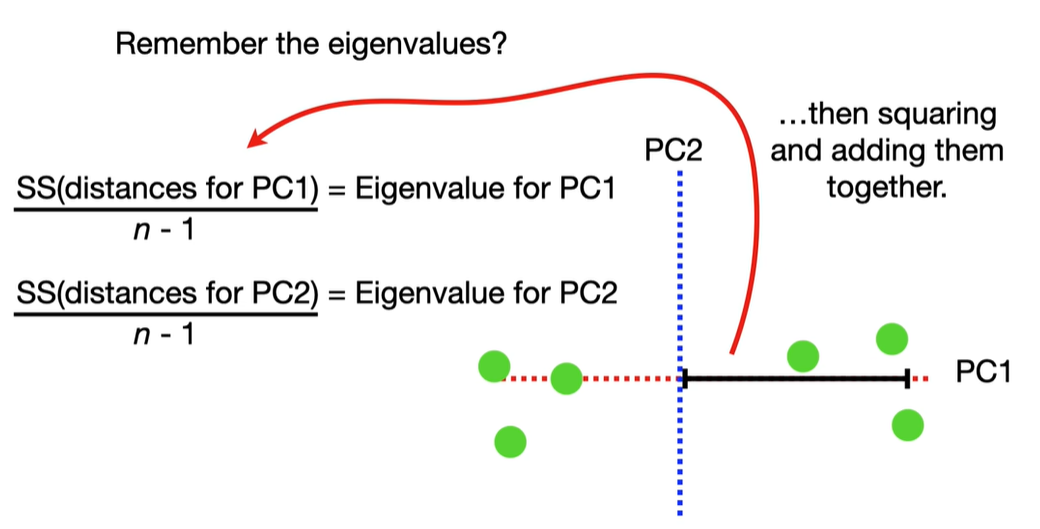
The reason we divide by n−1n - 1n−1 instead of nnn in Step 2 (when computing the covariance matrix in PCA) is because we're computing the sample covariance matrix, not the population covariance matrix.

🔍 Here's the key difference:

• Divide by nnn → for population covariance (when you have all possible data points).

• Divide by n−1n - 1n−1 → for sample covariance (when you're working with a sample drawn from a larger population).

---

📌 Why divide by n−1n - 1n−1 for samples?

This adjustment is known as Bessel’s correction, and it's used to make the sample variance (and hence the sample covariance) an unbiased estimator of the true population variance/covariance.

Without Bessel's correction:

This tends to underestimate the true covariance.

With Bessel's correction:

This is unbiased, meaning the expected value of the sample covariance equals the true population covariance.

---

🧠 In PCA:

Since PCA is usually applied to a sample dataset (not the entire population), we use:

This ensures that the eigenvalues correctly reflect the variance structure of the sample data.

 

 

 

 

 

    rotating 90 degree means multiplying i: (4+i)*i = -1+4i

 

 

 

 

 

 

 

     

 

      

 

 

     

 

     

 

 

 

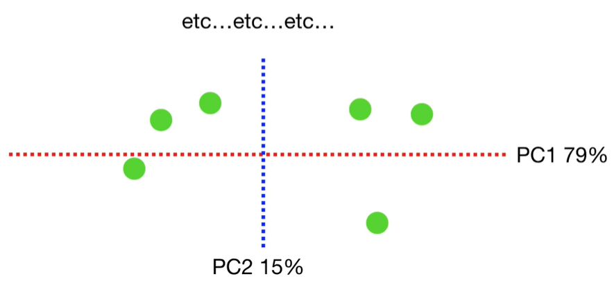
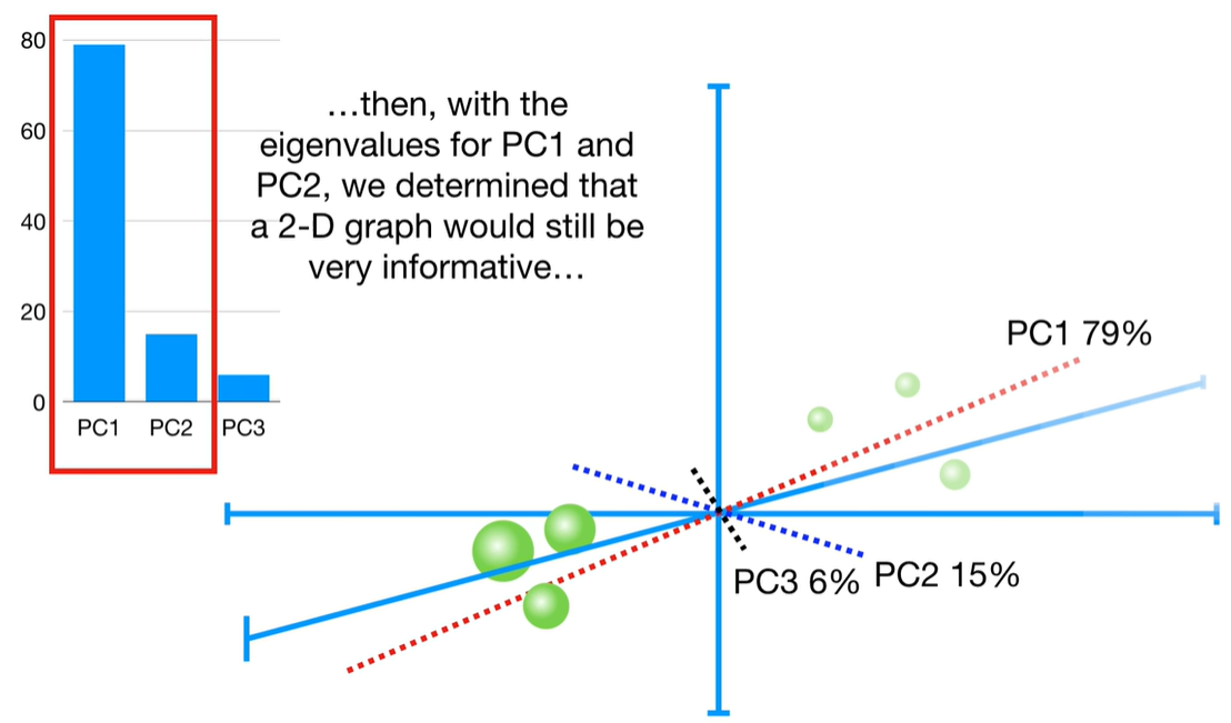
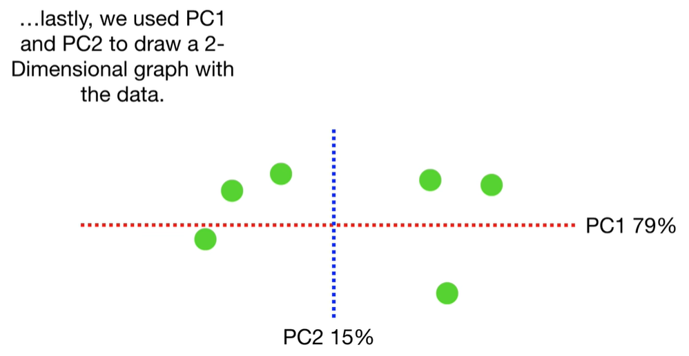
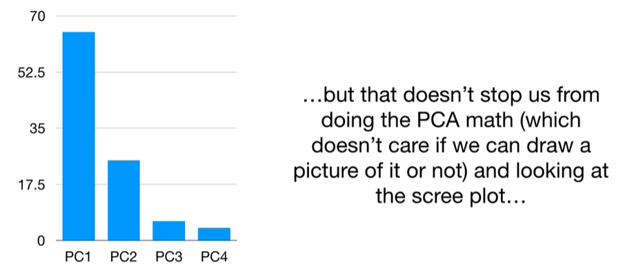
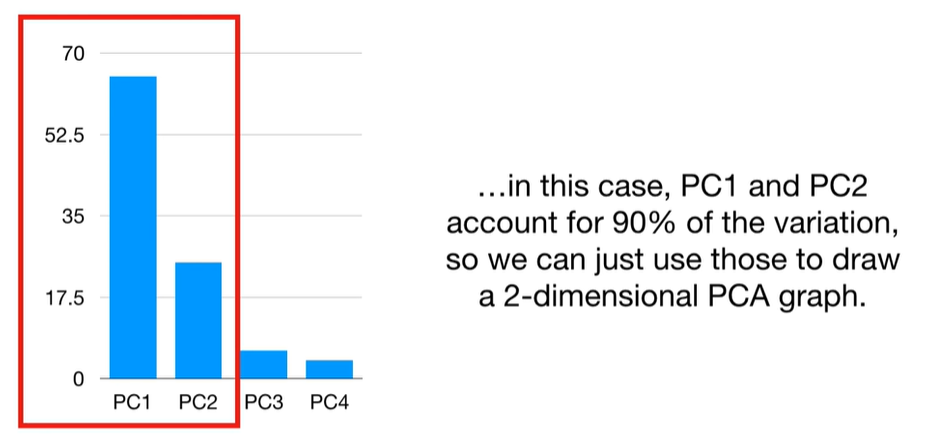
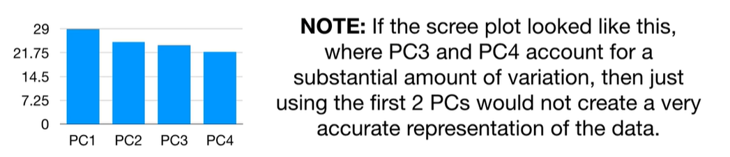
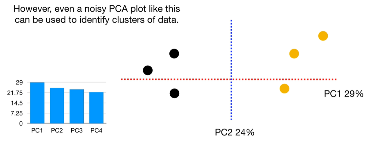
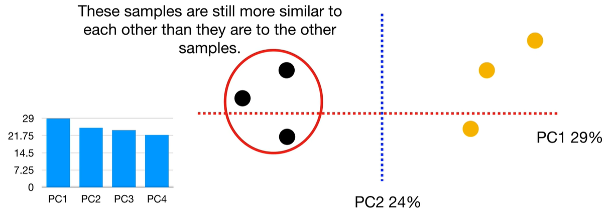
     scree plot