


The correlation coefficient is a numerical measure that describes the strength and direction of a linear relationship between two variables.
The Most Common: Pearson Correlation Coefficient (r)
It measures how closely two variables X and Y are linearly related.

Given two variables:
-
X=[x1,x2,...,xn]
-
Y=[y1,y2,...,yn]
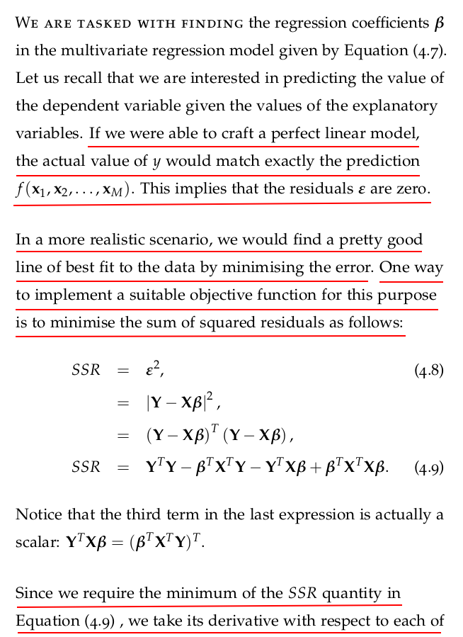
The formula is:

Interpretation of r
| r value | Interpretation |
|---|---|
| 1 | Perfect positive correlation |
| 0.7 to 0.9 | Strong positive correlation |
| 0.3 to 0.7 | Moderate positive correlation |
| 0 to 0.3 | Weak positive correlation |
| 0 | No correlation |
| -1 to 0 | Same as above, but negative |
import numpy as np

# Example data
x = [1, 2, 3, 4, 5]
y = [2, 4, 5, 4, 5]

# Calculate correlation coefficient
r = np.corrcoef(x, y)[0, 1]

print("Correlation coefficient:\n", r)
Correlation coefficient:
 [[1.         0.77459667]
 [0.77459667 1.        ]]
 regression

✅ What is Regression?
Regression is a statistical method used to model and analyze the relationship between a dependent variable (target) and one or more independent variables (features).
Its goal is to predict or estimate the value of the dependent variable based on the input(s).
🔢 Basic Example
Imagine you want to predict someone’s weight based on their height.
-
Height = independent variable (input)
-
Weight = dependent variable (output)
Regression helps us find a line or curve that best fits this relationship.
📈 Types of Regression
-
Linear Regression
Models the relationship as a straight line.
Formula:![]()
Where:
-
y: predicted value
-
x: input
-
m: slope
-
b: intercept
-
-
Multiple Linear Regression
Uses more than one input variable:![]()
-
Polynomial Regression
Models non-linear relationships using polynomials:![]()
-
Logistic Regression (Despite its name, it's used for classification)
Predicts probabilities, e.g., whether an email is spam or not.


📊 What Regression Tells You
-
Direction: Does yyy increase or decrease with xxx?
-
Strength: How strong is the relationship?
-
Prediction: What’s the likely yyy for a new xxx?
🧠 Machine Learning Context
In machine learning, regression algorithms are used when the output is a continuous value.
Example:
-
Predicting house prices
-
Forecasting sales
-
Estimating temperature


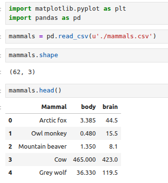
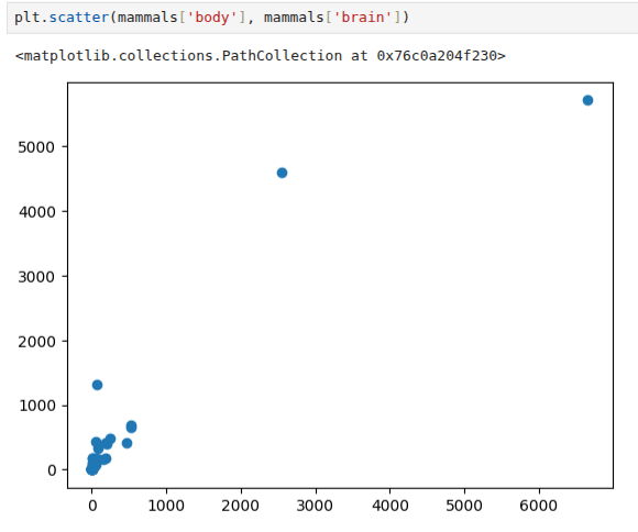
4.4 Brain and Body: Regression with One Variable
The dataset that we will use looks at the relationship of the body mass of an animal and the mass of its brain4 . The data is available at http: //dx.doi.org/10.6084/m9.figshare.1565651 as well as at http://www.statsci.org/data/general/sleep.html.
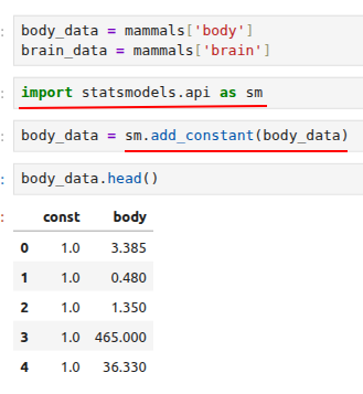
We are ready to run our regression with the ordinary least squares (OLS) method implemented in statsmodels:
regression1 = sm.OLS(brain_data, body_data).fit()
If you are familiar with R, you are probably familiar with the “formula notation” used to refer to the dependency of a variable on appropriate regressors. So, if you have a function y = f ( x ), in R you can denote that dependency with the use of a tilde, i.e., ~. This is an easy way to deal with denoting the dependency among variables, and fortunately statsmodels has an API that allows us to make use of it in Python too:
import statsmodels.formula.api as smf

regression2 = smf.ols(data=mammals, formula='brain ~ body').fit()
Please note that the R-style formula does not require us to add the column of 1s to the independent variable. The regression coefficients obtained with both methods are the same, and do not forget that the .fit() command is needed in both cases.
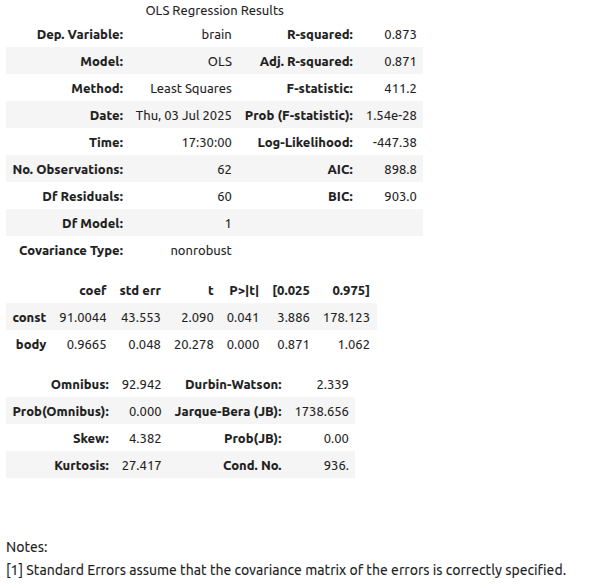
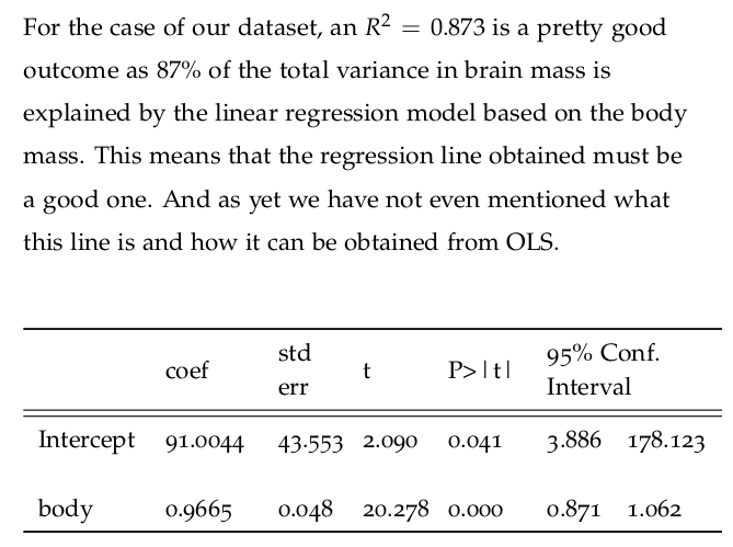
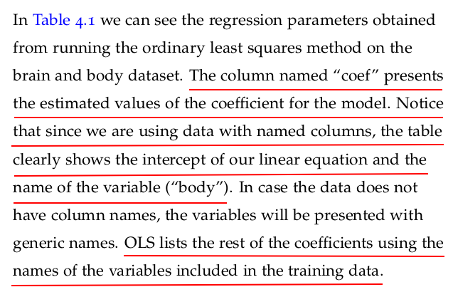
Let us now take a look at the results of fitting the model to the data provided. Statsmodels provides a summary method that renders a nice-looking table with the appropriate information.
regression1.summary()

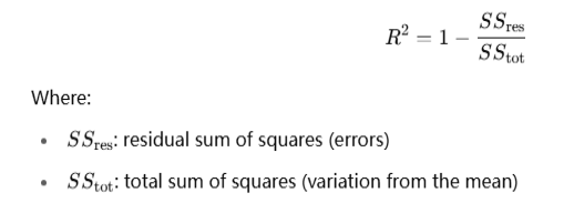
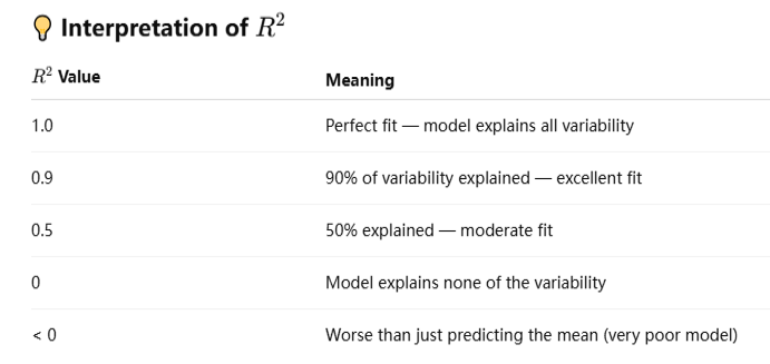
The coefficient of determination, commonly known as R2 (R-squared), is a key metric in regression analysis that tells you how well your model explains the variability in the dependent variable.
✅ Definition

🧪 Python Example (using sklearn)
from sklearn.linear_model import LinearRegression
from sklearn.metrics import r2_score

# Example data
X = [[1], [2], [3], [4], [5]]
y = [2, 4, 5, 4, 5]

model = LinearRegression()
model.fit(X, y)
predictions = model.predict(X)

r2 = r2_score(y, predictions)
print("R-squared:", r2)
Adjusted R2 — it improves on regular R2, especially when you have multiple predictors.
✅ What is Adjusted R2?
Adjusted R2 compensates for the fact that adding more variables to a regression will always increase (or keep) R2, even if those variables are useless.
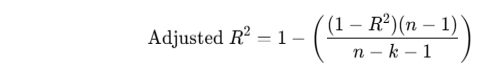
Where:
-
R2: the regular coefficient of determination
-
n: number of observations
-
k: number of independent variables
🔍 Why Use Adjusted R2?
-
Penalizes unnecessary variables
-
More reliable for model comparison when you have multiple features
-
Can decrease when you add unhelpful predictors
🧪 Python Example
Here’s a code example with multiple input variables and adjusted R2 manually calculated:
import numpy as np
from sklearn.linear_model import LinearRegression
from sklearn.metrics import r2_score

# Sample data: 3 features (X1, X2, X3) and 1 target (y)
X = np.array([
    [1, 2, 3],
    [2, 3, 4],
    [3, 4, 5],
    [4, 5, 6],
    [5, 6, 7]
])

y = np.array([2, 4, 5, 4, 5])

# Fit the model
model = LinearRegression()
model.fit(X, y)
y_pred = model.predict(X)

# R-squared
r2 = r2_score(y, y_pred)

# Adjusted R-squared
n = X.shape[0]  # number of samples
k = X.shape[1]  # number of predictors

adjusted_r2 = 1 - ((1 - r2) * (n - 1) / (n - k - 1))

print("R-squared:", r2)
print("Adjusted R-squared:", adjusted_r2)
It is very similar to R2 , but it introduces a penalty as extra variables are included in the model. The adjusted R2 value increases only in cases where the new input actually improves the model more than would be expected by pure chance.
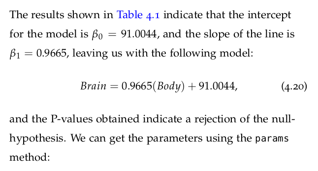
We can use this equation to predict the brain mass of a mammal given its body mass, and this can easily be done with the predict method in OLS. Let us consider new body mass measurements that will be used to predict the brain mass using the model obtained above. We need to prepare the new data in a way that is compatible with the model. We can therefore create an array of ten new data inputs as follows:
new_body = np.linspace(0, 7000, 10)
If we used the formula API to train our model, the predict method does not require us to add a column of 1s to our data, and instead we simply indicate that the new data points are going to be treated as a dictionary to replace the independent variable (i.e., exog in statsmodels parlance) in the fitted model. In other words, you can type the following commands:
brain_pred = regression2.predict(exog=dict(body=new_body))
print(brain_pred)
0      91.004396
1     842.723793
2    1594.443190
3    2346.162587
4    3097.881985
5    3849.601382
6    4601.320779
7    5353.040176
8    6104.759573
9    6856.478970
dtype: float64

The numbers shown correspond to the brain mass predictions for the artificial body mass measurements used as input. In Figure 4.4 we can see the regression line given by Equation (4.20) in comparison to the data points in the set. Please note that if you are not using the formula API, the input data will require the addition of a column of 1s to obtain the intercept.

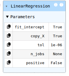
4.4.1 Regression with Scikit-learn
We have seen how to use statsmodels to perform our linear regression. One of the reasons to use this module is the user-friendly output it generates. Nonetheless, this is not the only way available to us to perform this analysis. In particular, Scikit-learn is another very useful module, and one that we use extensively throughout the book. For completeness, in this section we will see how to perform linear regression with Scikit-learn.
from sklearn import linear_model

body_data = mammals['body']
brain_data = mammals['brain']

sk_regr = linear_model.LinearRegression()

sk_regr.fit(body_data, brain_data)
ValueError: Expected a 2-dimensional container but got <class 'pandas.core.series.Series'> instead. Pass a DataFrame containing a single row (i.e. single sample) or a single column (i.e. single feature) instead.
body_data = mammals[['body']]
brain_data = mammals[['brain']]

sk_regr.fit(body_data, brain_data)
print(sk_regr.coef_)
print(sk_regr.intercept_)
print(sk_regr.score(body_data, brain_data))
[[0.96649637]]
[91.00439621]
0.8726620843043331
new_body = np.linspace(0, 7000, 10)
new_body = new_body[:, np.newaxis]
brain_pred = sk_regr.predict(new_body)

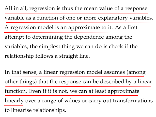
4.5 Logarithmic Transformation
One of the principal tenets of the linear regression model is the idea that the relationship between the variables at play is linear. In cases when that is not necessarily true, we can apply manipulations or transformations to the data that result in having a linear relationship. Once the linear model is obtained, we can then undo the transformation to obtain our final model.
A typical transformation that is often used is applying a logarithm to either one or both of the predictive and response variables.
Let us see what happens to the scatter plot of the body and brain data we have been analysing when we apply the logarithmic transformation to both variables. We will create a couple of new columns in our pandas dataframe to keep track of the transformations performed:
mammals['log_body'] = np.log(mammals['body'])
mammals['log_brain'] = np.log(mammals['brain'])
We can plot the transformed data, and as we can see from Figure 4.5 the data points are aligned in a way that indicates a linear relationship in the transformed space.
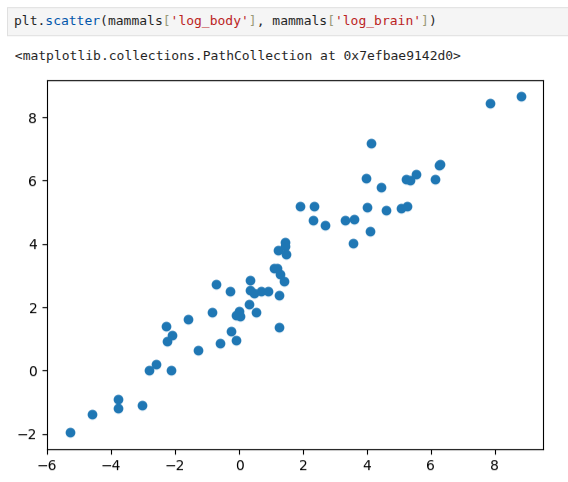
Why has this happened? Well, remember that we are trying to use models (simple and less simple ones) that enable us to exploit the patterns in the data. In this case, the relationship we see in this data may be modelled as a power law; e.g., y = xb .
The log-log transformation applied to the data maps this nonlinear relationship to a linear one, effectively transforming the complicated problem into a simpler one:

where we are using the notation log for the inverse of the exponential function e. As we can see, we have transformed our power law model, a nonlinear model in the regressor, into a form that looks linear as shown in Equation (4.22).
Now that we have this information at hand, we can train a new model using the transformed features attached to the mammals dataframe:
log_lm = smf.ols(formula='log_brain ~ log_body', data=mammals).fit()

The logarithmic transformation has increased the value of R2 from 0.873 to 0.921. We can see the value of the sum of squared residuals with the following command:
log_lm.ssr

# np.float64(28.92271042146064)
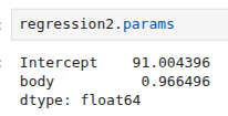
Let us now take a look at the statistics for the model as well as the all-important coefficients. As we can see from Table 4.2, the new model has an intercept of β0 = 2.1348 and a slope of β1 = 0.7517. The regression line for this model can be seen in Figure 4.6.

Remember that the coefficients obtained above are for the transformed data. If we wanted to relate this to the original features, we would need to undo the transformation. In this case we have a model given by

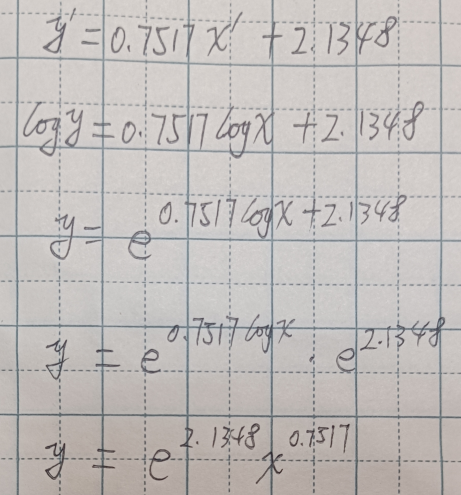
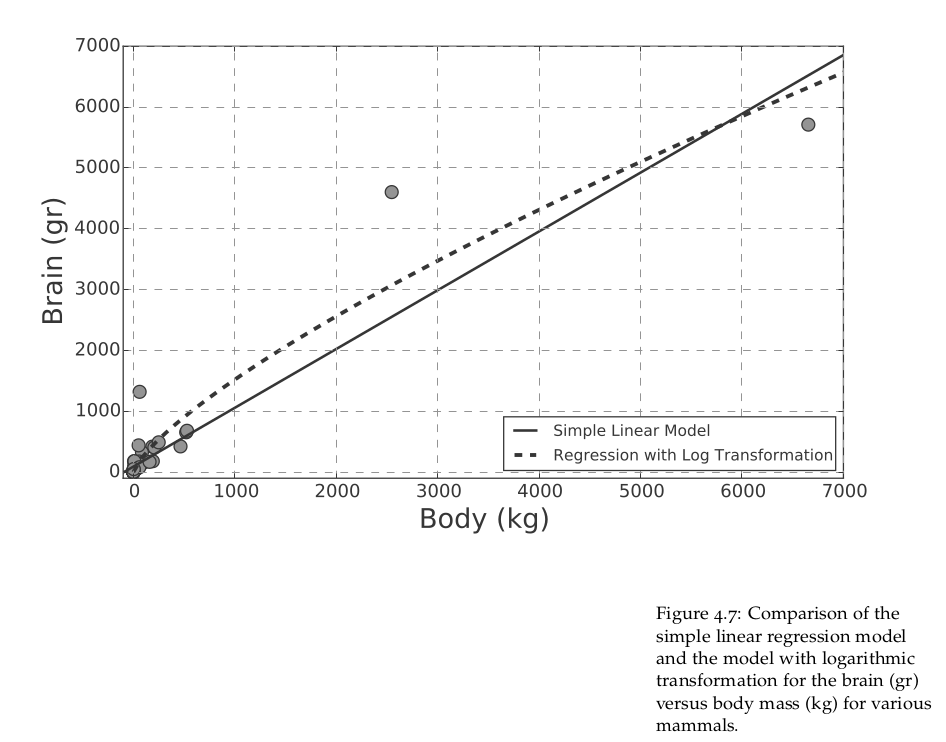
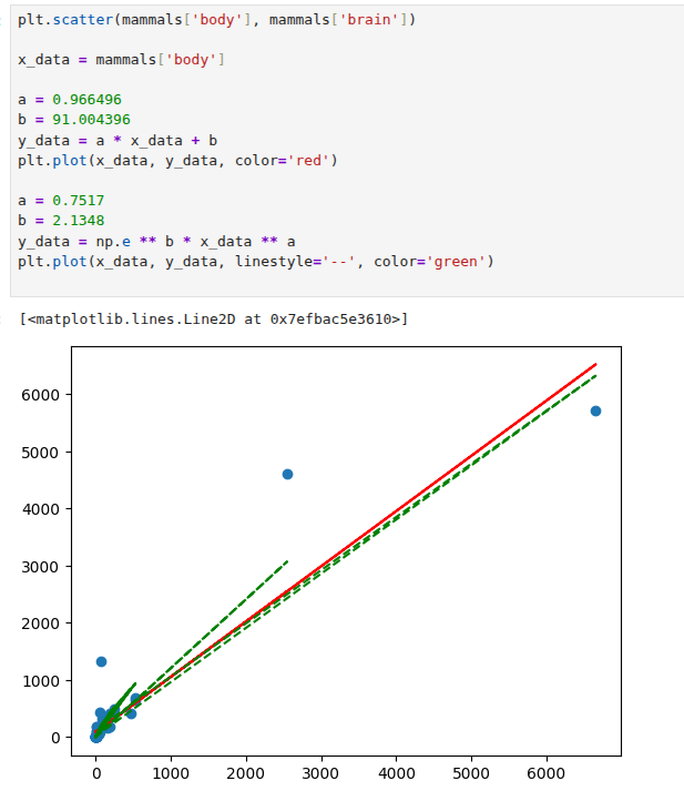
In Figure 4.7 we can see the original scatter plot and a comparison of the two models. It is easy to see how the logarithmic transformation allows for greater flexibility, capturing those data points which are a struggle for the simple linear model. This comparison demonstrates that it is possible to build a variety of models to explain the behaviour we observe in the data. In Section 4.7 we will see how we can fit a polynomial regression to the same dataset. Nonetheless, please remember that carrying out appropriate splitting of training and testing sets, together with cross-validation, is an unrivalled way to decide which model, among those tried, is the most suitable to use with unseen data.
4.6 Making the Task Easier: Standardisation and Scaling
In this section we are going to present a couple of the most widely used techniques to transform our data and provide us with anchors to interpret our results.
One of those techniques consists on centring the predictors such that their mean is zero, and it is often used in regression analysis. Among other things, it leads to interpreting the intercept term as the expected value of the target variable when the predictors are set to zero. Another useful transformation is the scaling of our variables. This is convenient in cases where we have features that have very different scales, where some variables have large values and others have very small ones.
As mentioned above, standardisation and scaling may help us interpret our results: They allow us to transform the features into a comparable metric with a known range, mean, units and/or standard deviation. It is important to note that the transformations to be used depend on the dataset and the domain where the data is sourced from and applied to. It also depends on the type of algorithm and answer sought. For example, in a comprehensive study of standardisation for cluster analysis, Milligan and Cooper7 report that standardisation approaches that use division by the range of the feature provide a consistent recovery of clusters. We shall talk about clustering in the next chapter. Let us go through the two techniques mentioned above in a bit more detail.
4.6.1 Normalisation or Unit Scaling
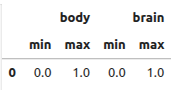
The aim of this transformation is to convert the range of a given variable into a scale that goes from 0 to 1. Given a feature f with a range between fmin and fmax the transformation is given by:

Notice that this method of scaling will cast our features into equal ranges, but their means and standard deviations will be different.
We can apply this unit scaling to our data with the preprocessing method in Scikit-learn that includes the MinMaxScaler function to implement unit scaling.
from sklearn import preprocessing

scaler = preprocessing.MinMaxScaler()

mammals_minmax = pd.DataFrame(scaler.fit_transform(mammals[['body', 'brain']]), columns=['body', 'brain'])
mammals_minmax.groupby(lambda idx: 0).agg(['min', 'max'])
4.6.2 z-Score Scaling
An alternative method for scaling our features consists of taking into account how far away data points are from the mean. In order to provide a comparable measure, the distance from the mean is calculated in units of the standard deviation of the feature data.
In this case a positive score tells us that a given data point is above the mean, whereas a negative one is below the mean. The standard score explained above is called the z-score as it is related to the normal distribution. The transformation that we need to carry out for a feature f with mean µf and standard deviation σf is given by:

Strictly speaking, the z-score must be calculated with the mean and standard deviation of the population; otherwise, we are making use of Student’s t statistic.
Scikit-learn’s pre-processing method allows us to standardise our features in a very straightforward manner:
scaler2 = preprocessing.StandardScaler()

mammals_std = pd.DataFrame(scaler2.fit_transform(mammals[['body', 'brain']]), columns=['body', 'brain'])
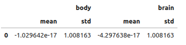
After the transformation we should have features with 0 mean and standard deviation 1; let us check that this is the case:
mammals_std.groupby(lambda idx: 0).agg(['mean', 'std'])
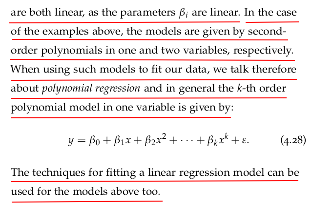
4.7 Polynomial Regression

Let us fit a quadratic model to the brain and body dataset we have been using in the previous sections. We can start by adding a feature that corresponds to the square of the body mass:
mammals['body_squared'] = mammals['body'] ** 2
We can now fit the quadratic model given by Equation (4.26), and using statsmodels is a straightforward task:
poly_reg = smf.ols(data=mammals, formula='brain ~ body + body_squared').fit()
We can take a look at the parameters obtained:
print(poly_reg.params)
Intercept       19.115299
body             2.123929
body_squared    -0.000189
dtype: float64
In other words, we have a model given by

It may seem that the coefficient of the quadratic term is rather small, but it does make a substantial difference to the predictions. Let us take a look by calculating the predicted values and plot them against the other two models:
new_body = np.linspace(0, 7000, 10)
new_body = new_body[:, np.newaxis]

poly_brain_pred = poly_reg.predict(exog=dict(body=new_body, body_squared=new_body**2))
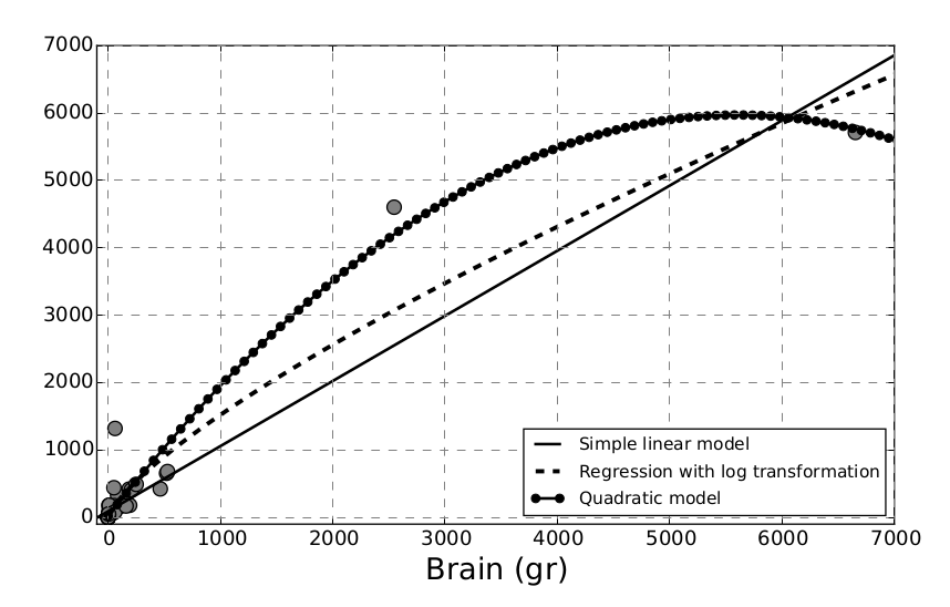
As we can see in Figure 4.8, the polynomial regression captures the data points much closer than the other two models. However, by increasing the complexity of our model, we are running the risk of overfitting the data. We know that cross-validation is a way to avoid this problem, and other techniques are at our disposal, such as performing some feature selection by adding features one at a time (forward selection) or discarding non-significant ones (backward elimination). In Section 4.9 we shall see how feature selection can be included in the modelling stage by applying regularisation techniques.
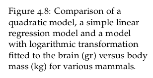
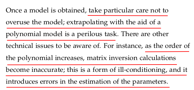
When using polynomial regressions, there are a number of things that should be taken into account. For instance, the order of the polynomial model should be kept as low as possible; remember that we are trying to generalise and not run an interpolation.
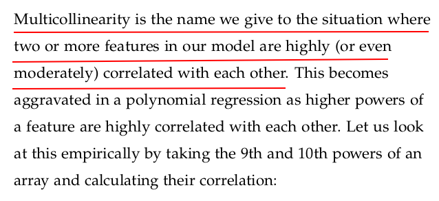
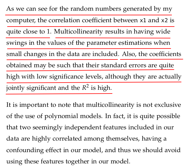
Multicollinearity refers to a situation in multiple regression analysis where two or more independent variables (predictors) are highly correlated with each other. This means that one predictor can be linearly predicted from the others with a substantial degree of accuracy.
Why is multicollinearity a problem?
Multicollinearity doesn't reduce the predictive power or reliability of the entire model, but it does affect the individual predictors:
-
Unstable Coefficients: Small changes in the data can lead to large swings in coefficient estimates.
-
Inflated Standard Errors: Confidence intervals for coefficients become wide, making it hard to determine which variables are statistically significant.
-
Reduced Interpretability: It's difficult to assess the individual impact of each predictor variable.
Signs of Multicollinearity
-
High correlation coefficients between predictor variables.
-
High Variance Inflation Factor (VIF) values (typically, VIF > 5 or 10 indicates a problem).
-
Regression coefficients that change significantly when you add or remove a variable.
Example
Suppose you have a model to predict house prices using both house size in square feet and number of rooms. These two variables are likely to be highly correlated (larger houses tend to have more rooms), which can cause multicollinearity.
How to Detect Multicollinearity
-
Correlation matrix: Examine the correlations between predictors.
-
VIF (Variance Inflation Factor): A common method to quantify how much multicollinearity exists.
from statsmodels.stats.outliers_influence import variance_inflation_factor
from statsmodels.tools.tools import add_constant
import pandas as pd

X = add_constant(df[['x1', 'x2', 'x3']])
vif = pd.DataFrame()
vif["VIF"] = [variance_inflation_factor(X.values, i) for i in range(X.shape[1])]
vif["feature"] = X.columns
print(vif)
How to Handle It
-
Remove one of the correlated variables.
-
Combine variables (e.g., via PCA or creating a composite score).
-
Regularization techniques like Ridge regression or Lasso.

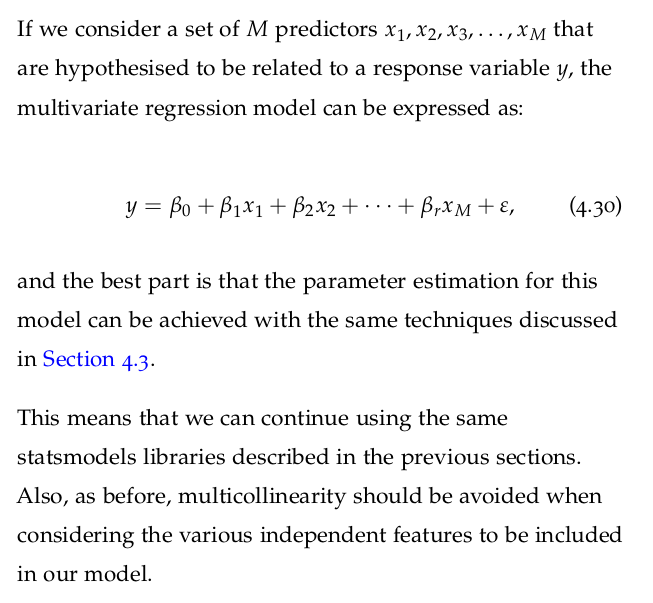
4.7.1 Multivariate Regression


 浙公网安备 33010602011771号