Data Science and Analytics with Python Study Notes 1

1.3 Data Science Tools

• Data framework: BigQuery, Spark, Databricks, Snowflake.

• Streaming data collection: Kafka, Flink, Amazon Kinesis.

• Job scheduling: Azkaban and Apache Oozie.

Tools for job scheduling are essential in orchestrating and managing workflows, ensuring that various tasks are executed in  a timely and coordinated manner. Azkaban is an opensource workflow management system developed at LinkedIn, designed to simplify the execution, monitoring, and dependency management of jobs. It allows users to define job dependencies graphically through a webbased user interface, making it user-friendly for workflow creation.

• NoSQL databases: MongoDB and Apache Cassandra.

For querying non-relational databases, several tools cater to the unique structures and requirements of these databases. MongoDB offers MongoDB Compass as a graphical user interface tool for visually exploring and querying data stored in MongoDB. Apache Cassandra has tools like DataStax DevCenter and CQL Shell for querying.

• Workflow management: Apache Airflow, Luigi, Prefect, Apache NiFi.

Tools for data science workflows are crucial for orchestrating and automating the various stages of the data science lifecycle. Apache Airflow stands out as a popular open-source platform for workflow automation and scheduling. Airflow allows data scientists to define, schedule, and monitor complex workflows as Directed Acyclic Graphs (DAGs). It integrates seamlessly with different data science tools, databases, and services, enabling the automation of tasks such as data extraction, transformation, model training, and deployment.

 

1.4 From Data to Insight: the Data Science Workflow

 

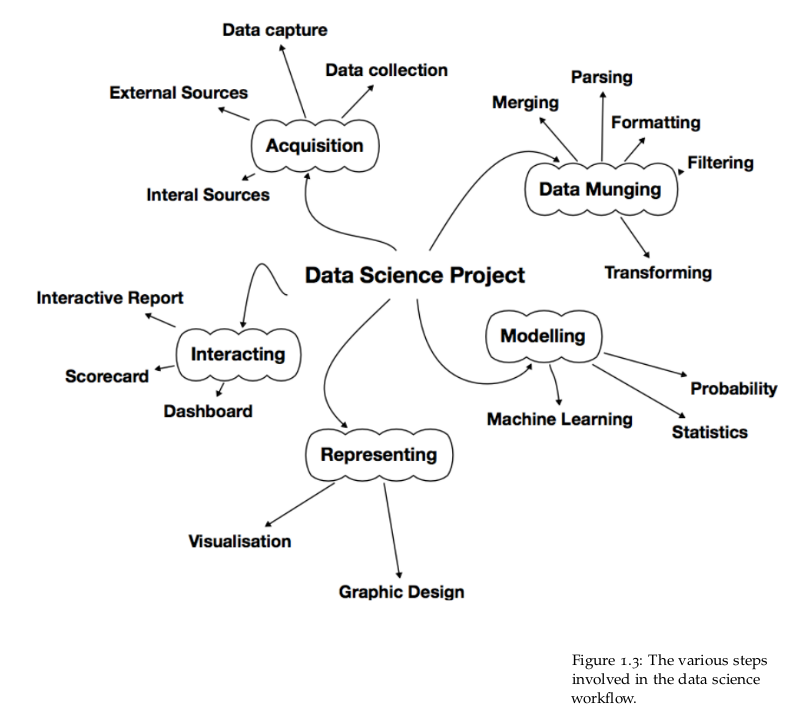
The various steps, shown in Figure 1.3, in the data science workflow include:

• Question identification

Without a clear question, there is no insight. Breaking down the problem into smaller questions is useful.

• Data acquisition

Once you have a problem to tackle, the first thing is figuring out if you or your organisation has the appropriate data that may be used to answer the question. If the answer is no, you will need to find appropriate sources for suitable data externally – web, social media, government, repositories, vendors, etc. Even in the case where the data is available internally, the data may be in locations that are hard to access due to technology, or even for regulatory and security reasons.

• Data munging

If there is no insight without a question, then there is no meaningful data without the process of data munging.  Data munging, also known as data wrangling, is the essential step of cleaning, transforming and organising raw data into a structured format suitable for analysis. This process is foundational in ensuring that the data used for any analytics or modeling is reliable, accurate, and relevant. Without thorough data preparation, the extraction of valuable insights becomes a near-impossible task. Munging is where one truly becomes intimately familiar with their dataset.

• Model construction

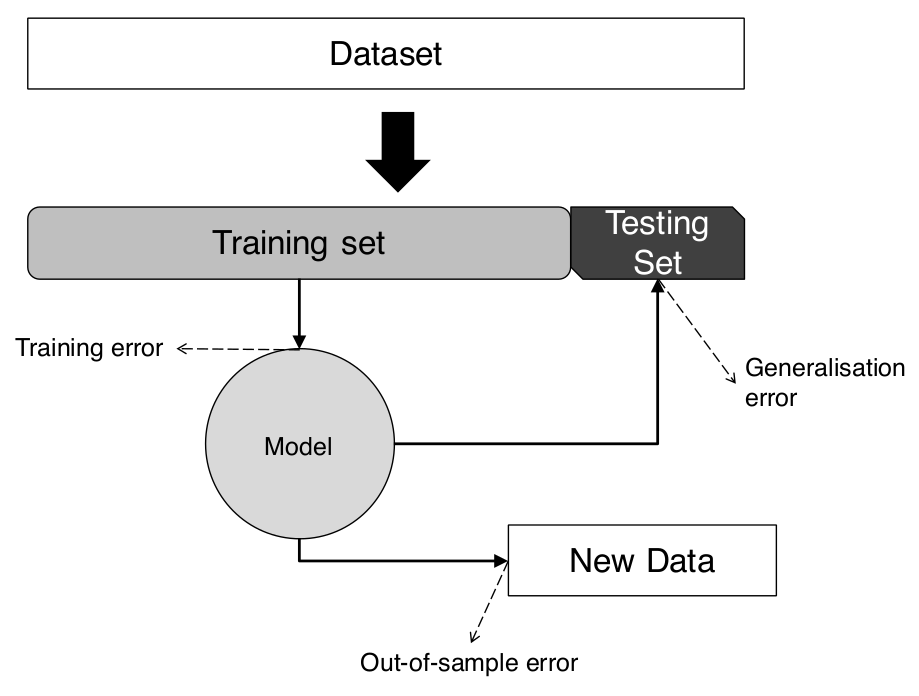
Having a clean dataset to feed to a machine learning or statistical model is a good start. Nonetheless, the question remains regarding what the most appropriate algorithm to use is. A partial answer to that question is that the best algorithm depends on the type of data you have, as well as its completeness. It also depends on the question you decided to tackle. Once the model has been run through the so-called training dataset, the next thing to do is to evaluate how effective and accurate the model is against the testing dataset and decide if the model is suitable for deployment. Every model needs to be evaluated.

• Representation

• Interaction

The fact that they have been listed in that order does not mean that they have to be followed one after the other. The workflow outlined above is not necessarily followed in sequence.

 

     L2-norm

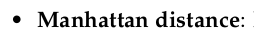
     L1-norm

 

 

 

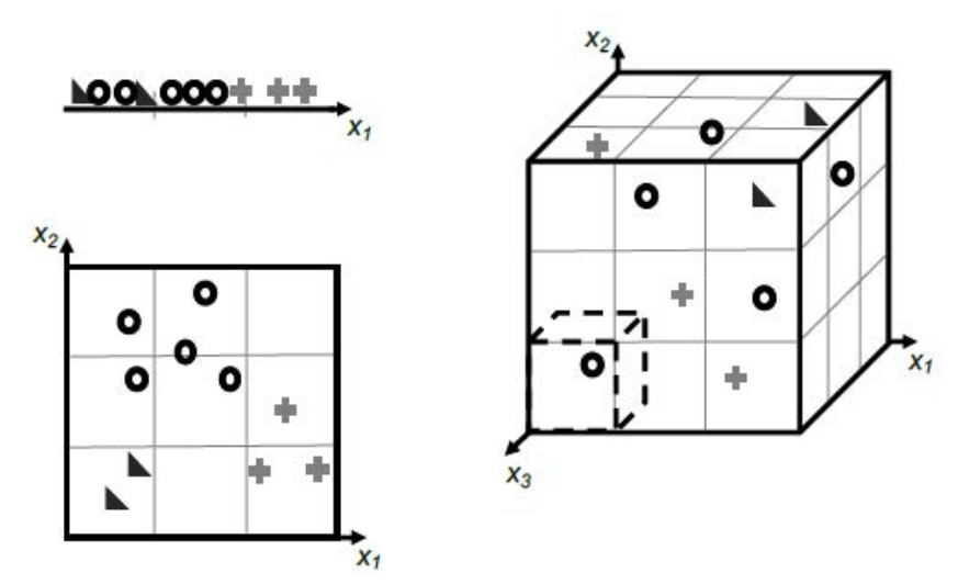
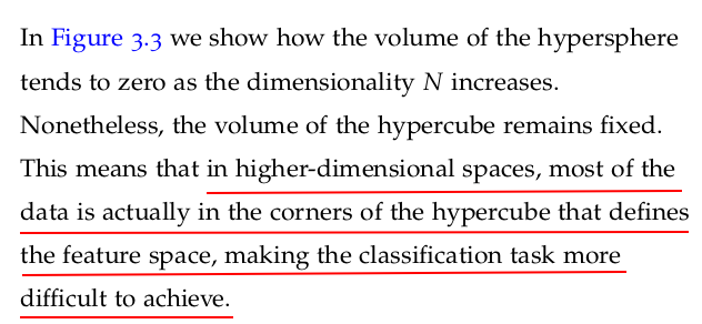
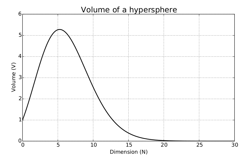
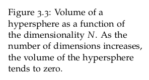
3.10 Beware the Curse of Dimensionality

It follows that as we increase the number of features, the number of dimensions that our model must include is increased too. Not only that, but we will also increase the amount of information required to describe the data instances, and therefore the model.

As the number of dimensions increases, we need to consider the fact that more data instances are required, particularly if we are to avoid overfitting. The realisation that the number of data points required to sample a space grows exponentially with the dimensionality of the space is usually called the curse of dimensionality.

The curse of dimensionality becomes more apparent in instances where we have datasets with a number of features much larger than the number of data points. We can see why this is the case when we consider the calculation of the distance between data points in spaces with increasing dimensionality.

     

 

 

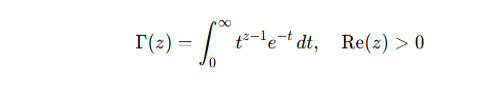
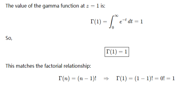
The gamma function, denoted by Γ(z)\Gamma(z)Γ(z), is a mathematical function that generalizes the factorial function to complex and real number arguments, except for the non-positive integers.

Definition:

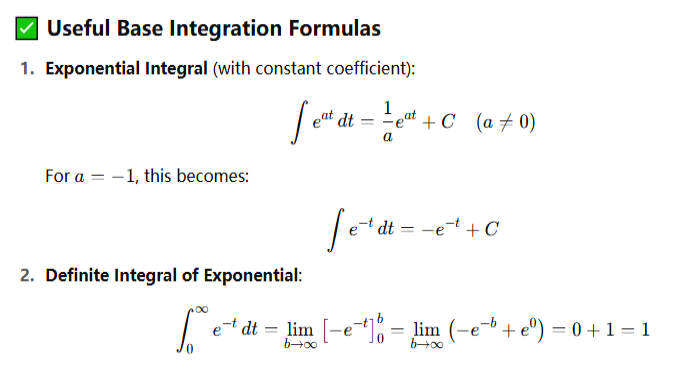
For a complex number zzz with a positive real part, the gamma function is defined by the improper integral:

Key Properties:

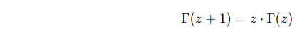
1. Relation to factorial:

   
   

2. Recursive property:

   
   

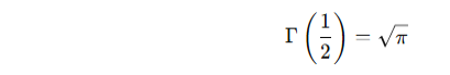
3. Value at 1/2:

   
   

4. Analytic continuation:
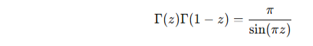
   The gamma function is defined for all complex numbers except the non-positive integers (i.e., 0,−1,−2,…0, -1, -2, \dots0,−1,−2,…), where it has simple poles.

5. Euler's reflection formula:

   
   

Applications:

• Probability and statistics (e.g., gamma distribution, beta distribution)

• Complex analysis

• Differential equations

• Physics and engineering problems

 

 

 

     

 

 

     

 

 

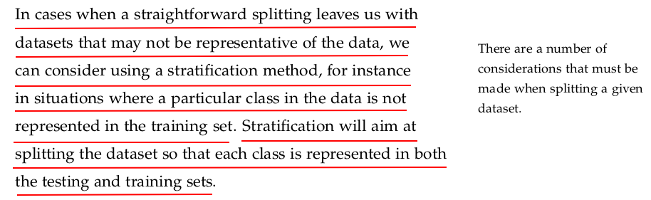
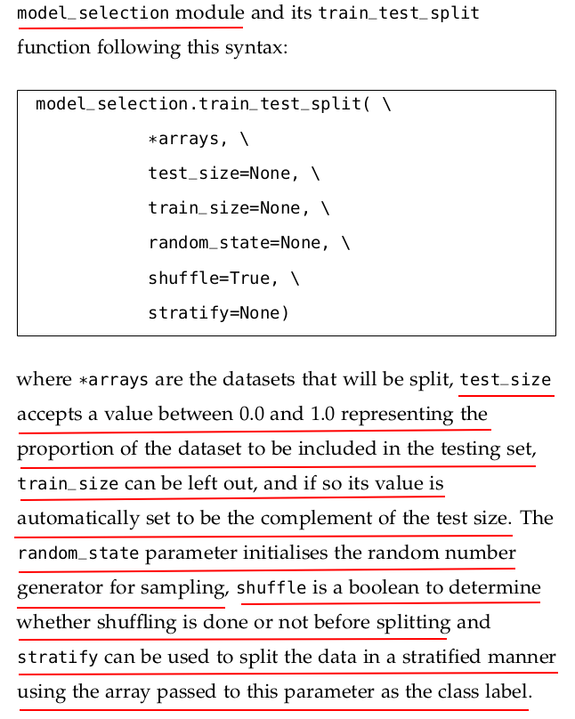
The stratify parameter in sklearn.model_selection.train_test_split is used to ensure that the class distribution in the target variable is preserved when splitting the dataset into training and test sets.

This is especially useful for classification problems with imbalanced classes, so that both the training and test sets have similar class proportions.

📌 Example:

Let's say we have a binary classification problem with an imbalanced dataset:

from sklearn.model_selection import train_test_split
import numpy as np
from collections import Counter

# Sample features (just placeholder numbers)
X = np.arange(100).reshape((50, 2))  # 50 samples, 2 features each

# Labels: Imbalanced dataset (40 of class 0, 10 of class 1)
y = np.array([0]*40 + [1]*10)

# Without stratification
X_train, X_test, y_train, y_test = train_test_split(X, y, test_size=0.2, random_state=42)
print("Without stratify:", Counter(y_test))

# With stratification
X_train_s, X_test_s, y_train_s, y_test_s = train_test_split(X, y, test_size=0.2, random_state=42, stratify=y)
print("With stratify:   ", Counter(y_test_s))

🧾 Output:

Without stratify: Counter({0: 9, 1: 1})
With stratify:    Counter({0: 8, 1: 2})

 

Here's an example using a real-world dataset: breast_cancer from sklearn.datasets. We'll use stratify=y with train_test_split to ensure the malignant/benign class distribution remains consistent in both the training and test sets.

from sklearn.datasets import load_breast_cancer
from sklearn.model_selection import train_test_split
from collections import Counter

# Load the dataset
data = load_breast_cancer()
X = data.data
y = data.target  # 0 = malignant, 1 = benign

# Print overall class distribution
print("Original class distribution:", Counter(y))

# Split without stratification
X_train1, X_test1, y_train1, y_test1 = train_test_split(X, y, test_size=0.2, random_state=42)
print("Test set without stratify: ", Counter(y_test1))

# Split with stratification
X_train2, X_test2, y_train2, y_test2 = train_test_split(X, y, test_size=0.2, random_state=42, stratify=y)
print("Test set with stratify:    ", Counter(y_test2))

🧾 Output (approximate numbers):

Original class distribution: Counter({1: 357, 0: 212})
Test set without stratify:  Counter({1: 77, 0: 37})
Test set with stratify:     Counter({1: 72, 0: 43})

✅ As you can see, using stratify=y maintains the same class distribution (~63% benign, ~37% malignant) in the test set as in the full dataset.

 

 

 

     

 

 

from sklearn.datasets import load_breast_cancer
from sklearn.model_selection import KFold
from sklearn.linear_model import LogisticRegression
from sklearn.metrics import accuracy_score
import numpy as np

# Load the breast cancer dataset
data = load_breast_cancer()
X = data.data
y = data.target

# Set up KFold cross-validator
kf = KFold(n_splits=5, shuffle=True, random_state=42)

# Initialize model
model = LogisticRegression(max_iter=1000)

# Track accuracy for each fold
fold_accuracies = []

# K-fold cross-validation loop
for fold, (train_idx, test_idx) in enumerate(kf.split(X)):
    X_train, X_test = X[train_idx], X[test_idx]
    y_train, y_test = y[train_idx], y[test_idx]
    
    # Train the model
    model.fit(X_train, y_train)
    
    # Predict on test fold
    y_pred = model.predict(X_test)
    
    # Compute accuracy
    acc = accuracy_score(y_test, y_pred)
    fold_accuracies.append(acc)
    
    print(f"Fold {fold + 1}: Accuracy = {acc:.4f}")

# Average accuracy
print(f"\nAverage Accuracy over 5 folds: {np.mean(fold_accuracies):.4f}")