

PART III: INDUCTIVE LOGIC
Chapter 9: Analogy and Legal and Moral Reasoning
9.1 Analogical Reasoning
Analogical reasoning may be the most fundamental and the most common of all rational processes. It stands at the basis of many ordinary decisions in life. For example, a woman wanting to buy a can of soup might deliberate between Campbell’s and Brand X and, after recalling that other varieties of Campbell’s were good, decide in favor of that brand. A man contemplating a haircut might recall that a friend got an especially good cut at the Golden Touch and as a result decide to go there himself. A woman selecting a plant for her garden might observe that gardenias grow well at the house next door and conclude that gardenias would grow well at her house, too. A man thinking of reading a novel by Stephen King might recall that King’s last three novels were thrilling and conclude that his latest novel would also be thrilling.
Analogical reasoning is reasoning that depends on a comparison of instances. If the instances are sufficiently similar, the decision reached in the end is usually a good one; but if they are not sufficiently similar, the decision may not be good. When such a reasoning process is expressed in words, the result is an argument from analogy (see Chapter 1). Simple arguments from analogy have the following structure:

If the attributes a, b, and c are connected in some important way to z (that is, are relevant to z), the argument is usually strong. If they are not so connected (that is, are irrelevant to z), the argument is usually weak.
Analogical arguments are closely related to generalizations. In a generalization, the arguer begins with one or more instances and proceeds to draw a conclusion about all the members of a class. The arguer may then apply the generalization to one or more members of this class that were not noted earlier. The first stage of such an inference is inductive, and the second stage is deductive. For example, the man thinking of reading the latest Stephen King novel might argue that because the last three novels by King were thrilling, all King novels are thrilling (inductive argument). Applying this generalization to the latest novel, he might then conclude that it too will be thrilling (deductive argument).In an argument from analogy, on the other hand, the arguer proceeds directly from one or more individual instances to a conclusion about another individual instance without appealing to any intermediate generalization. Such an argument is purely inductive. Thus, the arguer might conclude directly from reading three earlier King novels that the latest one will be thrilling.
In any argument from analogy, the items that are compared are called analogues. Thus, if one should argue that Britney Spears’s latest CD is probably good because her two previous CDs were good, the three CDs are the analogues. The two earlier CDs are called the primary analogues, and the latest CD is called the secondary analogue. With these definitions in mind, we may now examine a set of principles that are useful for evaluating most arguments from analogy. They include (1) the relevance of the similarities shared by the primary and secondary analogues, (2) the number of similarities, (3) the nature and degree of disanalogy, (4) the number of primary analogues, (5) the diversity among the primary analogues, and (6) the specificity of the conclusion.
1. Relevance of the similarities. Suppose a certain person—let us call her Lucy—is contemplating the purchase of a new car. She decides in favor of a Chevrolet because she wants good gas mileage and her friend Tom’s new Chevy gets good gas mileage. To support her decision, Lucy argues that both cars have a padded steering wheel, tachometer, vinyl upholstery, tinted windows, CD player, and white paint. Lucy’s argument is weak because these similarities are irrelevant to gas mileage. On the other hand, if Lucy bases her conclusion on the fact that both cars have the same-size engine, her argument is relatively strong, because engine size is relevant to gas mileage.
2. Number of similarities. Suppose, in addition to the same-size engine, Lucy notes further similarities between the car she intends to buy and Tom’s car: curb weight, aerodynamic body, gear ratio, and tires. These additional similarities, all of which are relevant to gas mileage, tend to strengthen Lucy’s argument. If, in addition, Lucy notes that she and Tom both drive about half on city streets and half on freeways, her argument is strengthened even further.
3. Nature and degree of disanalogy. On the other hand, if Lucy’s car is equipped with a turbocharger, if Lucy loves to make jackrabbit starts and screeching stops, if Tom’s car has overdrive but Lucy’s does not, and if Lucy constantly drives on congested freeways while Tom drives on relatively clear freeways, Lucy’s argument is weakened. These differences are called disanalogies. Depending on how they relate to the conclusion, disanalogies can either weaken or strengthen an argument. If we suppose instead that Tom’s car has the turbocharger, that Tom loves jackrabbit starts, and so on, then Lucy’s argument is strengthened, because these disanalogies tend to reduce Tom’s gas mileage.
4. Number of primary analogues. Thus far, Lucy has based her conclusion on the similarity between the car she intends to buy and only one other car—Tom’s. Now suppose that Lucy has three additional friends, that all of them drive cars of the same model and year as Tom’s, and that all of them get good gas mileage. These additional primary analogues strengthen Lucy’s argument because they lessen the likelihood that Tom’s good gas mileage is a freak incident. On the other hand, suppose that two of these additional friends get the same good gas mileage as Tom but that the third gets poor mileage. As before, the first two cases tend to strengthen Lucy’s argument, but the third now tends to weaken it. This third case is called a counteranalogy because it supports a conclusion opposed to that of the original analogy.
5. Diversity among the primary analogues. Suppose now that Lucy’s four friends (all of whom get good mileage) all buy their gas at the same station, have their cars tuned up regularly by the same mechanic, put the same friction-reducing additive in their oil, inflate their tires to the same pressure, and do their city driving on uncongested, level streets at a fuel-maximizing 28 miles per hour. Such factors would tend to reduce the probability of Lucy’s conclusion, because it is possible that one or a combination of them is responsible for the good mileage and that this factor (or combination of them) is absent in Lucy’s case. On the other hand, if Lucy’s friends buy their gas at different stations, have their cars tuned up at different intervals by different mechanics, inflate their tires to different pressures, drive at different speeds on different grades, and have different attitudes toward using the oil additive, then it is less likely that the good gas mileage they enjoy is attributable to any factor other than the model and year of their car.
6. Specificity of the conclusion. Lucy’s conclusion is simply that her car will get “good” mileage. If she now changes her conclusion to state that her car will get gas mileage “at least as good” as Tom’s, then her argument is weakened. Such a conclusion is more specific than the earlier conclusion and is easier to falsify. Thus, if her mileage were only one-tenth of a mile per gallon less than Tom’s, her conclusion would turn out to be false. Now suppose that Lucy changes her conclusion to state that her car will get exactly the same gas mileage as Tom’s. This conclusion is even more specific than the “at least as good” conclusion, and it is easier still to falsify. Thus, such a conclusion renders Lucy’s argument much weaker than her original argument.
Let us now use these six principles to evaluate an argument from analogy. Suppose that you want to shade a bedroom window from the intense western sun. To accomplish this purpose, you decide to plant some trees, but the trees must be narrow ones that will grow approximately 25 feet tall. Recalling that a friend has some Italian cypresses that are almost exactly 25 feet tall, you conclude that this variety of tree will do the job. Thus far, your argument is based on a single similarity, the species of the tree. Because this similarity is very relevant to height, your argument is fairly strong. Now if, in addition, it turns out that your friend lives in the same city and has the same kind of soil as you, your argument is strengthened. However, if it happens that your friend has a knack for growing trees while you have a knack for killing them, your argument is weakened.
To this set of facts, suppose we add the observation that four of your neighbors have Italian cypresses and that all of their trees are approximately 25 feet tall. This fact tends to strengthen your argument. Also, if all four neighbors planted their trees in different years, use different kinds of fertilizers on them, and give them different amounts of water, your argument is further strengthened. Finally, should you broaden your conclusion to state that your trees will grow between 22 and 28 feet tall, your argument is strengthened even further. But if you narrow your conclusion to state that your trees will grow to between 24.5 and 25.5 feet tall, your argument is weakened.
9.2 Legal Reasoning
Many of the arguments used by lawyers in the United States and Canada to support a case at trial are analogical arguments. The reason is that the legal systems of these countries were derived many years ago from the English system, and an essential feature of the English system is its dependence on precedent. According to the requirement of precedent, similar cases must be decided similarly. Thus, in arguing a case, a lawyer will often attempt to show that the case is analogous to some earlier case that was decided in a favorable way. Sometimes, even today, these precedents go back to early English law.
For example, suppose you own a factory and one of your machines, a drill press, breaks down, causing the entire operation to come to a halt. Urgently you call a repair company and explain the whole situation. The spokesperson for the company promises to have the drill press back in operation within two days. Unfortunately, there are delays, and two weeks elapse before the drill press is repaired. In the meantime your company loses an additional $10,000 in profits. Because you relied on the spokesperson’s assurance that the drill press would be fixed in two days, you demand that the repair company reimburse you for the additional lost profits. When the repair company refuses your demand, you file suit.
The lawyer who argues your case will probably make reference to a much earlier case, Hadley v. Baxendale, decided in Gloucester, England, in 1854. In that case the operation of a mill was halted because of a broken crankshaft, and the owner of the mill (Hadley) employed a shipping company (Baxendale) to return the crankshaft to the manufacturer. Hadley informed Baxendale that the broken crankshaft had interrupted the operation of the mill, and Baxendale replied that the broken crankshaft would be in the hands of the manufacturer within one day. As it turned out, the shipment was delayed by several days, and Hadley incurred lost profits from the additional time the mill was shut down. Hadley demanded reimbursement from Baxendale, and when Baxendale refused, Hadley filed suit. The court ruled that Baxendale should pay only if he foresaw when he agreed to do the work that delays would result in lost profits for Hadley.
Applying this result to the drill press case, your lawyer will argue that because the repair company was informed that delays in repairing the drill press would result in lost profits, it should reimburse you for the losses incurred.
In the early days, much of English law resulted directly from judges’ rendering decisions in particular cases. This judge-made law is otherwise called common law. However, today many of our laws are not the direct product of judges but rather of legislative bodies. These laws, called statutes, are codified in books that are periodically revised. Can it be said that precedent plays a central role in decisions involving statutory law in the same way that it does in decisions involving common law? The answer is a definite yes. Statutory laws are invariably phrased in relatively general language, and precedent is required to determine how the statutes should be interpreted and applied.
Consider, for example, a “law” that we are all familiar with, the First Amendment to the U.S. Constitution, which provides for freedom of speech and religious expression. Suppose that you decide, in reliance on the First Amendment, to pass out religious pamphlets on a downtown street corner. Suppose further that most of the people you hand your pamphlets to merely glance at them and then throw them on the street and that the gathering litter makes the area look like a garbage dump. To prevent the litter, the police tell you that you can hand out your pamphlets only in the vicinity of public garbage cans, so that those who do not want the pamphlets can properly dispose of them. You object that such a restriction violates your First Amendment rights, and you take the issue to court.
In presenting your case, your lawyer will argue that the case is analogous to other cases where the state attempted to limit not the content of religious expression, but the time, place, and manner of its expression. Next, your lawyer will note that in such cases the state is allowed to restrict the expression only if the restriction is “narrowly tailored” to serve a “significant government interest.” Finally, your lawyer will attempt to show that your case is analogous to cases in which the government failed to prove that the restriction was so tailored.
As these examples illustrate, many of the arguments that occur in law are arguments from analogy, and the principles developed at the beginning of this section can be used to evaluate them. The first principle, which deals with the relevance of the similarities, has an obvious application to legal arguments. Suppose, for example, that two cases are similar in that each involves a burning building, the building in each case is located in Chicago, and in each case ten people died. The comparison is pointless if the issue in the first case is whether an insurance company is liable to pay damages while the issue in the second is whether somebody is guilty of arson.
The second and third principles, which deal with the number of similarities and the nature and degree of disanalogy, are also applicable. If a preceding case resembles the case at hand in virtually all important details, then the preceding case is said to be “on point” and, given certain other requirements (discussed shortly), will dictate the outcome of the case to be decided. As for the nature and degree of disanalogy, if a preceding case deals with fraud by a stockbroker while the case to be decided deals with fraud by a real estate broker, the precedent may be more or less controlling, depending on such circumstances as applicable statutory law.
As applied to legal analogies, the fourth principle (number of primary analogues) usually determines how well established a legal precedent is. If fifty previous courts have followed a certain rule, the precedent is stronger (everything else being equal) than if only two courts have followed that rule. The fifth principle (diversity of primary analogues) is also applicable. If a certain rule turns up in a broad range of cases, it provides a stronger precedent (other things being equal) than a rule that turns up in a narrow range of cases. For example, the principle underlying the inadmissibility of hearsay testimony is well established because it appears in a broad cross section of cases.
Finally, the sixth principle states that the more specific a conclusion is, the weaker the argument becomes. Suppose, in an earlier case, a person is awarded half a million dollars for injuries inflicted by a surgeon who, during an appendix operation, left a stethoscope in the body opening. The argument that another person injured in the same way by another doctor should be awarded exactly the same amount of money is relatively weak in comparison with the argument that the person should be awarded approximately the same amount of money.
Analogical arguments that occur in law differ from the fairly simple analogies considered earlier in at least two important ways. In the analogy dealing with gas mileage, the modes of similarity that linked the analogues (number of engine cylinders, curb weight, and the like) were clearly defined by conventional thinking, and their relevance to the conclusion had been established by scientific principles. In law, however, clarity of this sort is seldom to be found. Modes of similarity between cases are often the result of highly creative thinking by lawyers and judges, and the relevance of these similarities to the proposed conclusion is nearly always debatable. These differences render analogical arguments in law considerably more elusive than those dealing with subjects such as gas mileage.
The other difference between simple analogical arguments and those found in law is that the primary analogues in law (earlier cases) do not all have equal weight. The reason is that our courts operate in different jurisdictions. The system of federal courts is totally separate from the system of state courts. As a result, a case that might have considerable weight as a precedent in one system might have little or no weight in the other. In addition, within these systems there are different circuits, and a case that is controlling in one circuit may not be in another. Lastly, within these systems, the courts exist on different levels. For example, within the federal system there are the district courts, courts of appeals, and the U.S. Supreme Court. A case that is binding on a lower court may not be binding on a higher court.
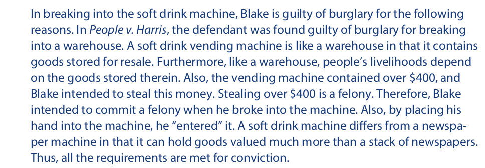
Let us now illustrate the process of legal reasoning with a hypothetical example. Suppose a certain vagrant—let us call him Blake—attempted to earn some pocket change by breaking into a soft drink vending machine and stealing the cash. The police apprehended Blake in the act, and the district attorney charged him with burglary. Blake had one prior conviction for breaking into a soft drink machine.
The first thing that any lawyer would do with this case is to recall the definition of “burglary.” According to the traditional definition, “burglary” means “the trespassory breaking and entering of a dwelling house of another at night with the intent to commit a felony therein.” Under many modern statutes, “dwelling house” has been replaced by “structure” and “at night” has been deleted.
There is little doubt that Blake has broken into a structure. The question is, is a soft drink machine the kind of structure intended by the statute? A second question is, did Blake intend to commit a felony when he broke into the soft drink machine? To answer these questions a lawyer would consult additional statutes and relevant cases. Let us suppose that our jurisdiction has a statute that defines felony theft as theft of $400 or more. Also, let us suppose that the cash box of this particular machine contained $450 but most similar machines can hold no more than $350.
As for cases, let us suppose that our jurisdiction has two controlling precedents. In People v. Harris, Harris broke into a warehouse with the intent of stealing its contents. The warehouse contained microwave ovens valued at $10,000, and Harris was found guilty of burglary. In People v. Sawyer, Sawyer broke into a newspaper vending machine with the intent to steal the cash in the cash box. The maximum capacity of the cash box was $20, and Sawyer was found not guilty of burglary.
Relying on these facts and preceding cases, the district attorney might present the following argument to the judge (or jury):
Defense counsel, on the other hand, might argue as follows:
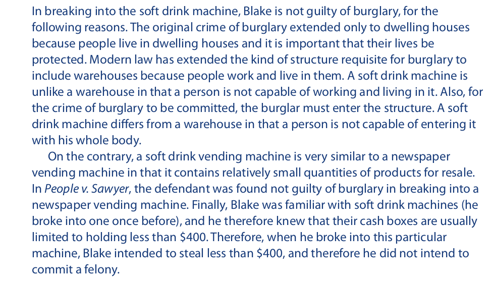
In deciding whether Blake is guilty, the judge or jury will have to evaluate these analogical arguments by determining which analogies are the strongest.
Sometimes lawyers and judges are confronted with cases for which there is no clear precedent. Such cases are called cases of first impression, and the attempt to deal with them by appeal to analogous instances involves even more creativity than does the attempt to deal with ordinary cases. In deciding cases of first impression, judges often resort to moral reasoning, and they grope for any analogy that can shed light on the issue. The reasoning process in such a decision often involves a sequence of analogies followed by disanalogies and counteranalogies. These analogies present the issue in a continually shifting light, and the experience of coming to grips with them expands the outlook of the reasoner. New perspectives are created, attitudes are changed, and worldviews are altered.
9.3 Moral Reasoning
As in law, arguments from analogy are also useful in deciding moral questions. Such arguments often occur in the context of a dialogue. As an example of a dialogue that includes several arguments from analogy, consider the following one between two fictional characters, Jason and Deirdre. The dialogue deals with the morality and legality of fetal abuse.

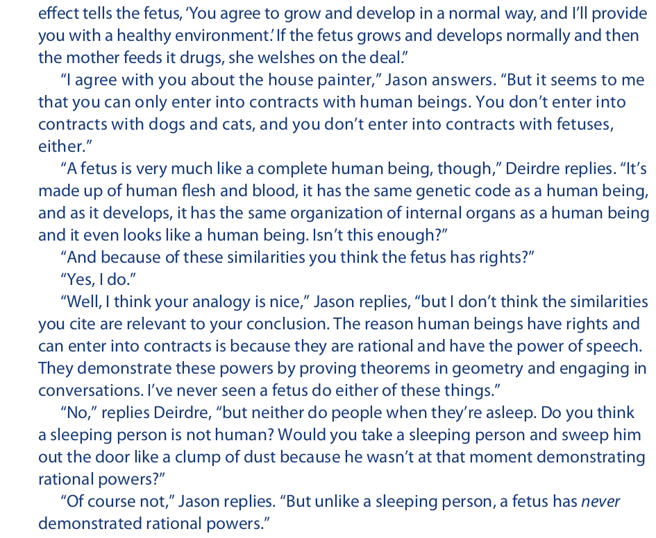
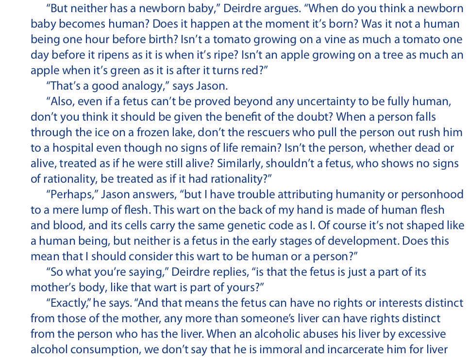
This dialogue contains numerous analogies and counteranalogies. The modes of similarity between the many primary analogues and the secondary analogues (the fetus, women who commit fetal abuse, laws against fetal abuse, and so on) are never relevant beyond dispute, and the nature and degree of disanalogy rarely has undisputed consequences. However, the dialogue serves to illustrate the subtle effect that analogies have on our thought processes and the power they have to alter our attitudes and perspectives.
Chapter 10: Causality and Mill's Methods
10.1 “Cause” and Necessary and Sufficient Conditions
A knowledge of causal connections plays a prominent role in our effort to control the environment in which we live. We insulate our homes because we know insulation will prevent heat loss, we vaccinate our children because we know vaccination will protect them from polio and diphtheria, we practice the piano and violin because we know that by doing so we may become proficient on them, and we cook our meat and fish because we know that doing so will make them edible.
When the word “cause” is used in ordinary English, however, it is seriously affected by ambiguity. For example, when we say that sprinkling water on the flowers will cause them to grow, we mean that water is required for growth, not that water alone will do the job—sunshine and the proper soil are also required. On the other hand, when we say that taking a swim on a hot summer day will cause us to cool off, we mean that the dip by itself will do the job, but we understand that other things will work just as well, such as taking a cold shower, entering an air-conditioned room, and so on.
To clear up this ambiguity affecting the meaning of “cause,” adopting the language of sufficient and necessary conditions is useful. When we say that electrocution is a cause of death, we mean “cause” in the sense of sufficient condition. Electrocution is sufficient to produce death, but there are other methods equally effective, such as poisoning, drowning, and shooting. On the other hand, when we say that the presence of clouds is a cause of rain, we mean “cause” in the sense of necessary condition. Without clouds, rain cannot occur, but clouds alone are not sufficient. Certain combinations of pressure and temperature are also required.
Sometimes “cause” is used in the sense of necessary and sufficient condition, as when we say that the action of a force causes a body to accelerate or that an increase in voltage causes an increase in electrical current. For a body to accelerate, nothing more and nothing less is required than for it to be acted on by a net force; and for an electrical current to increase through a resistive circuit, nothing more and nothing less is required than an increase in voltage.
Thus, as these examples illustrate, the word “cause” can have any one of three different meanings:
1. Sufficient condition
2. Necessary condition
3. Sufficient and necessary condition
Sometimes the context provides an immediate clue to the sense in which “cause” is being used. If we are trying to prevent a certain phenomenon from happening, we usually search for a cause that is a necessary condition, and if we are trying to produce a certain phenomenon, we usually search for a cause that is a sufficient condition. For example, in attempting to prevent the occurrence of smog around cities, scientists try to isolate a necessary condition or group of necessary conditions that, if removed, will eliminate the smog. And in their effort to produce an abundant harvest, farmers search for a sufficient condition that, given sunshine and rainfall, will increase crop growth.
Another important point is that whenever an event occurs, at least one sufficient condition is present and all the necessary conditions are present. The conjunction of the necessary conditions is the sufficient condition that actually produces the event. For example, the necessary conditions for lighting a match are heat (produced by striking) and oxygen. Combining these two necessary conditions gives the sufficient condition. In other words, striking the match in the presence of oxygen is sufficient to ignite it. In cases where the sufficient condition is also a necessary condition, there is only one necessary condition, which is identical with the sufficient condition.
We can now summarize the meaning of cause in the sense of a sufficient condition and a necessary condition:

According to these statements, if A occurs and B does not occur, then A is not a sufficient condition for B, and if B occurs and A does not occur, then A is not a necessary condition for B. Thus:

These results will serve as important rules in the material that follows.
10.2 Mill’s Five Methods
In his System of Logic, the nineteenth-century philosopher John Stuart Mill compiled five methods for identifying causal connections between events. These he called the method of agreement, the method of difference, the joint method of agreement and difference, the method of residues, and the method of concomitant variation. In the years that have elapsed since the publication of Mill’s Logic, the five methods have received a good deal of philosophical criticism. Today most logicians agree that the methods fall short of the claims made for them by Mill, but the fact remains that the methods function implicitly in many of the inductive inferences we make in ordinary life.
In addition to criticizing these methods, modern logicians have introduced many variations that have multiplied their number beyond the original five. Some of these variations have resulted from the fact that Mill himself failed to distinguish causes that are sufficient conditions from causes that are necessary conditions. The account that follows introduces this distinction into the first three methods, but apart from that, it remains faithful to Mill’s own presentation.
Method of Agreement
Suppose that five people eat dinner in a certain restaurant, and a short while later all five become sick. Suppose further that these people ordered an assortment of items from the menu, but the only food that all of them ordered was vanilla ice cream for dessert. In other words, all of the dinners were in agreement only as to the ice cream. Such a situation suggests that the ice cream caused the sickness. The method of agreement consists in a systematic effort to find a single factor (such as the ice cream) that is common to several occurrences for the purpose of identifying that factor as the cause of a phenomenon present in the occurrences (such as the sickness).
The method of agreement identifies a cause in the sense of a necessary condition. To see how this method works, let us develop the restaurant example a bit further.
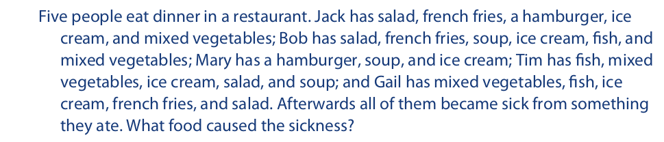
If we let occurrences 1 through 5 stand for Jack, Bob, Mary, Tim, and Gail, respectively, and let A through G represent salad, soup, french fries, a hamburger, fish, ice cream, and mixed vegetables, respectively, we can construct a table that reflects what these five people ate (Table 10.1). In this table an asterisk means that a certain food was eaten, and a dash means that it was not eaten.
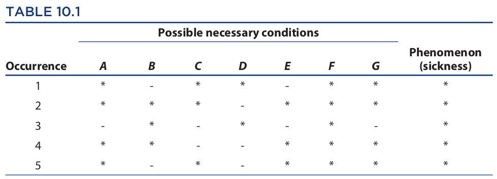
Now, since the method of agreement identifies a cause in the sense of a necessary condition, we begin by eliminating from this table the conditions that are not necessary for the occurrence of the phenomenon. In doing so, we use the rule that a condition is not necessary for the occurrence of a phenomenon if that condition is absent when the phenomenon is present. Thus, occurrence 1 eliminates condition B and condition E; occurrence 2 eliminates D; occurrence 3 eliminates A, C, E (again), and G; occurrence 4 eliminates C (again) and D (again); and occurrence 5 eliminates B (again) and D (again). This leaves only F (the ice cream) as a possible necessary condition. The conclusion is therefore warranted that the ice cream caused the sickness of the diners.
This conclusion follows only probably for two reasons. First, it is quite possible that some condition was overlooked in compiling conditions A through G. For example, if the ice cream was served with contaminated spoons, then the sickness of the diners could have been caused by that condition and not by the ice cream. Second, if more than one of the foods were contaminated (for example, both soup and french fries), then the sickness could have been caused by this combination of foods and not by the ice cream. Thus, the strength of the argument depends on the nonoccurrence of these two possibilities.
It is also important to realize that the conclusion yielded by Table 10.1 applies directly only to the five diners represented in the five occurrences, and not to everyone who may have eaten in the restaurant. Thus, if some food other than those listed in the table—for example, spaghetti—was contaminated, then only if they avoided both spaghetti and ice cream could the other diners be assured of not getting sick. But if, among all the foods in the restaurant, only the ice cream was contaminated, the conclusion would extend to the other patrons as well. This last point illustrates the fact that a conclusion reached by the method of agreement has limited generality. It applies directly only to those occurrences listed, and only indirectly, through a second inductive inference, to others.
Furthermore, because the conclusion yields a cause in the sense of a necessary condition, it does not assert that anyone who ate the ice cream would get sick. Many people have a natural immunity to food poisoning. What the conclusion says is that patrons who did not eat the ice cream would not get sick—at least not from the food. Thus, the method of agreement has a certain limited use. Basically what it says, in reference to the example, is that the ice cream is a highly suspect factor in the sickness of the patrons, and if investigators want to track down the cause of the sickness, this is where they should begin.
An example of an actual use of the method of agreement is provided by the discovery of the beneficial effects of fluoride on teeth. It was noticed several decades ago that people in certain communities were favored with especially healthy teeth. In researching the various factors these communities shared, scientists discovered that all had a high level of natural fluoride in their water supply. The scientists concluded from this evidence that fluoride causes teeth to be healthy.
Method of Difference
For an example of how this method works, let us modify our earlier case of people becoming sick from eating food in a restaurant. Instead of five people, suppose that identical twins, who have identical susceptibilities to food poisoning, go to that restaurant for dinner. They both order identical meals except that one orders ice cream for dessert while the other does not. The ice cream is the only way that the two meals differ. Later the twin who ordered the ice cream gets sick, whereas the other twin does not. The natural conclusion is that the ice cream caused the sickness.
The method of difference consists in a systematic effort to identify a single factor that is present in an occurrence in which the phenomenon in question is present, and absent from an occurrence in which the phenomenon is absent. The method is confined to investigating exactly two occurrences, and it identifies a cause in the sense of a sufficient condition. For a clearer illustration of how this method works, let us add a few details to the twin example:
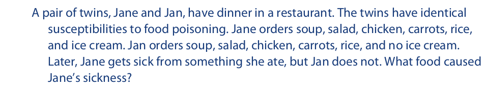
If we let Jane and Jan stand for occurrences 1 and 2, respectively, and let A stand for the specific susceptibility to food poisoning shared by Jane and Jan, and B through G stand for soup, salad, chicken, carrots, rice, and ice cream, respectively, we can produce Table 10.2. Again, an asterisk indicates that a certain condition is present, and a dash indicates it is absent.
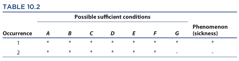
As with the method of agreement, we proceed to eliminate certain conditions, but in this case we use the rule that a condition is not sufficient for the occurrence of a phenomenon if it is present when the phenomenon is absent. Accordingly, occurrence 2 eliminates A, B, C, D, E, and F. This leaves only G as the sufficient condition for the phenomenon. Thus, G (ice cream) is the cause of Jane’s sickness.
Since the result yielded by the method of difference applies to only the one occurrence in which the phenomenon is present (in this case, Jane), it is often less susceptible to generalization than is the method of agreement, which usually applies to several occurrences. Thus, the mere fact that the ice cream may have caused Jane to become sick does not mean that it caused other patrons who ate ice cream to get sick. Perhaps these other people have a higher resistance to food poisoning than Jane or Jan. But given that the others are similar to Jane and Jan in relevant respects, the result can often be generalized to cover these others as well. At the very least, if others in the restaurant became sick, the fact that the ice cream is what made Jane sick suggests that this is where investigators should begin when they try to explain what made the others sick.
The conclusion yielded by the method of difference is only probable, however, even for the one occurrence to which it directly applies. The problem is that it is impossible for two occurrences to be literally identical in every respect but one. The mere fact that two occurrences occupy different regions of space, that one is closer to the wall than the other, amounts to a difference. Such differences may be insignificant, but therein lies the possibility for error. It is not at all obvious how insignificant differences should be distinguished from significant ones. Furthermore, it is impossible to make an exhaustive list of all the possible conditions; but without such a list there is no assurance that significant conditions have not been overlooked.
The objective of the method of difference is to identify a sufficient condition among those that are present in a specific occurrence. Sometimes, however, the absence of a factor can count as something positive that must be taken into account. Suppose, for example, that both of the twins who dined in the restaurant are allergic to dairy products, but they can avoid an allergic reaction by taking Lactaid tablets. Suppose further that both twins ordered ice cream for dessert, but only Jan took the tablets. After the meal, Jane got sick. We can attribute Jane’s sickness to the absence of the Lactaid.
We can illustrate this situation by modifying Table 10.2 as follows. Let A stand for the allergy to dairy products, let B through G stand for the same foods as before, and let H stand for Lactaid tablets. Then ~H will stand for the absence of Lactaid (the symbol ~ means “not”). As before, let occurrence 1 stand for Jane, and occurrence 2 for Jan (see Table 10.3).
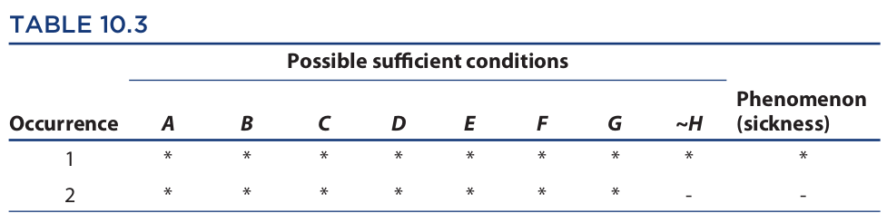
Using the same rule for elimination as with Table 10.2, we see that occurrence 2 eliminates A through G as sufficient conditions. This leaves ~H (the absence of Lactaid) as the cause of Jane’s sickness. In this case, the ice cream is not identified as the cause, because Jan (occurrence 2) ate ice cream (G) but did not get sick.
The method of difference has a wide range of applicability. For example, a farmer might fertilize one part of a field but not the other part to test the benefit of using fertilizer. If the fertilized part of the crop turns out to be fuller and healthier than the nonfertilized part, then the farmer can conclude that the improvement was caused by the fertilizer. On the other hand, a cook might leave some ingredient out of a batch of biscuits to determine the importance of that ingredient. If the biscuits turn out dry and crunchy, the cook can attribute the difference to the absence of that ingredient.
Joint Method of Agreement and Difference
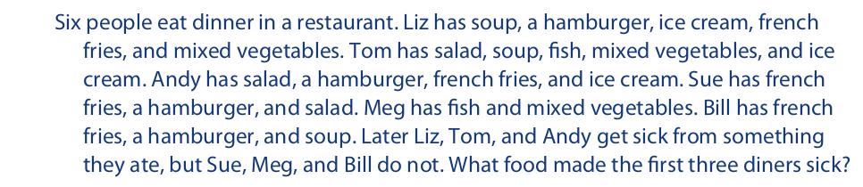
To illustrate the joint method, we can once again modify the example of the diners who got sick by eating food in a restaurant. In place of the original five diners and the pair of twins, suppose that six people eat dinner in the restaurant. Among the first three, suppose that a variety of meals are eaten but that only ice cream is consumed by all, and later all three get sick. And among the other three, suppose that a variety of meals are eaten but that none of these diners eats any ice cream, and later none of them gets sick. The conclusion is warranted that the ice cream is what made the first three diners sick.
The joint method of agreement and difference consists of a systematic effort to identify a single condition that is present in two or more occurrences in which the phenomenon in question is present and that is absent from two or more occurrences in which the phenomenon is absent, but never present when the phenomenon is absent nor absent when the phenomenon is present. This condition is then taken to be the cause of the phenomenon in the sense of a necessary and sufficient condition. To see more clearly how this method works, let us add some details to the example:
Let occurrences 1 through 6 stand for Liz, Tom, Andy, Sue, Meg, and Bill, respectively. And let A through G stand for salad, soup, a hamburger, fish, ice cream, french fries, and mixed vegetables (see Table 10.4).
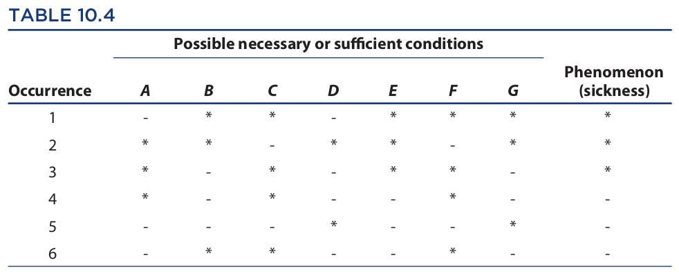
In the first three occurrences the phenomenon is present, so we proceed by eliminating possible necessary conditions. Using the rule that a condition is not necessary if it is absent when the phenomenon is present, occurrence 1 eliminates A and D, occurrence 2 eliminates C and F, and occurrence 3 eliminates B, D (again), and G. This leaves only E as the necessary condition. Next, in the last three occurrences the phenomenon is absent, so we use the rule that a condition is not sufficient if it is present when the phenomenon is absent. Occurrence 4 eliminates A, C, and F; occurrence 5 eliminates D and G; and occurrence 6 eliminates B, C (again), and F (again). This leaves only E as the sufficient condition. Thus, condition E (ice cream) is the cause in the sense of both a necessary and sufficient condition of the sickness of the first three diners.
Since the joint method yields a cause in the sense of both a necessary and sufficient condition, it is usually thought to be stronger than either the method of agreement by itself, which yields a cause in the sense of a necessary condition, or the method of difference by itself, which yields a cause in the sense of a sufficient condition. However, when any of these methods is used as a basis for a subsequent inductive generalization, the strength of the conclusion is proportional to the number of occurrences that are included. Thus, an application of the method of agreement that included, say, one hundred occurrences might offer stronger results than an application of the joint method that included, say, only six occurrences. By similar reasoning, multiple applications of the method of difference might offer stronger results than a single application of the joint method.
As with the other methods, the conclusion yielded by the joint method is only probable because some relevant condition may have been overlooked in producing the table. If, for example, both salad and soup were contaminated, then the ice cream could not be identified as a necessary condition for the sickness, and if one of the last three diners was naturally immune, then the ice cream could not be identified as a sufficient condition. Obviously the attempt to extend the results of this example to other patrons of the restaurant who may have gotten sick is fraught with other difficulties.
Lastly, we note that even though the name of the joint method suggests that it results from a mere combination of the method of agreement with the method of difference, this is not the case. Such a combination would consist of one occurrence in which the phenomenon is present, one occurrence in which the phenomenon is absent and which differs from the former occurrence as to only one condition, and one occurrence in which the phenomenon is present and which agrees with the first occurrence in only one condition. However, according to Mill, the joint method requires “two or more” occurrences in which the phenomenon is present, and “two or more” occurrences in which the phenomenon is absent.* His further description of the method accords with the foregoing account.
Method of Residues
This method and the one that follows are used to identify a causal connection between two conditions without regard for the specific kind of connection. Both methods may be used to identify conditions that are sufficient, necessary, or both sufficient and necessary. The method of residues consists of separating from a group of causally connected conditions and phenomena those strands of causal connection that are already known, leaving the required causal connection as the “residue.” Here is an example:

The method of residues as illustrated in this example may be diagramed as follows:
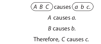
In reference to the draft example, A B C is the combination of possible conditions producing a b c , the total draft. When A (the broken window) is separated out, it is found to cause a (a portion of the draft). When B (the crack) is separated out, it is found to cause b (another portion of the draft). The conclusion is that C (the broken damper) causes c (the remaining portion of the draft). The conclusion follows only probably because it is quite possible that a fourth source of the draft was overlooked. Here is another example:
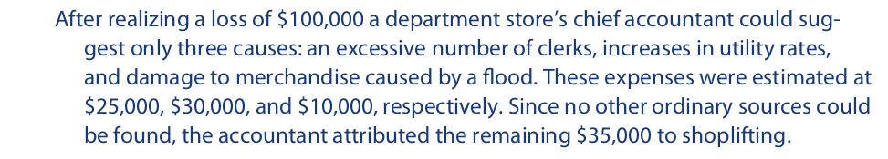
In this case A B C D is the combination of conditions consisting of the number of clerks, the utility rate increases, the flood, and shoplifting; and a b c d is the total loss of $100,000. After A, B, and C are separated out, the conclusion is that D (shoplifting) caused d (the remaining loss). Because the estimates might have been incorrect and because additional sources of financial loss might have been overlooked, the conclusion is only probable.
Some procedures that, at least on the face of it, appear to use the method of residues come closer to being deductive than inductive. A case in point is the procedure used to determine the weight of the cargo carried by a truck. First, the empty truck is put on a scale and the weight recorded. Then the truck is loaded and the truck together with the cargo is put on the same scale. The weight of the cargo is the difference between the two weights. If, to this procedure, we add the rather unproblematic assumptions that weight is an additive property, that the scale is accurate, that the scale operator reads the indicator properly, that the truck is not altered in the loading process, and a few others, the conclusion about the weight of the cargo follows deductively.
To distinguish deductive from inductive uses of the method of residues, we must take into account such factors as the role of mathematics. If the conclusion depends on a purely arithmetical computation, the argument is probably best characterized as deductive. If not, then it is probably inductive.
Method of Concomitant Variation
The method of concomitant variation identifies a causal connection between two conditions by matching variations in one condition with variations in another. According to one formulation, increases are matched with increases and decreases with decreases. Example:
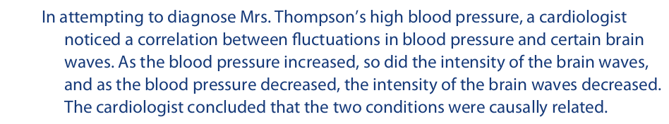
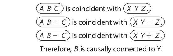
The method of concomitant variation as illustrated in this example may be diagramed as follows:
Here, A B C is a set of observable conditions such as cholesterol level, liver function, and basal metabolism, with B representing blood pressure; and X Y Z is another set of observable conditions with Y representing certain brain waves. In the second and third rows, B+ and B− represent increases and decreases in blood pressure, and Y+ and Y− represent increases and decreases in the intensity of the brain waves. The conclusion asserts that either B causes Y, Y causes B, or B and Y have a common cause. Determining which is the case requires further investigation; of course, if B occurs earlier in time than Y, then Y does not cause B, and if Y occurs earlier in time than B, then B does not cause Y.
The blood pressure example matches increases in one condition with increases in another. For an example that matches increases in one condition with decreases in another, consider the following:

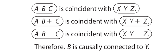
This second version of the method of concomitant variation may be diagramed as follows:
In this example A B C is a set of economic conditions such as stock exchange indexes, interest rates, and commodity prices, with B representing gross domestic product; and X Y Z is a set of social conditions such as birth rates, employment rates, and immigration numbers, with Y representing the national divorce rate. The conclusion is that B is somehow causally connected to Y. However, in this example an even stronger conclusion could probably be drawn—namely, that decreases in the GDP cause increases in the divorce rate, and not conversely. That changes in economic prosperity (which is indicated by GDP) should affect the divorce rate is quite plausible, but the converse is less so.
At this point we should note that the existence of a mere correlation between two phenomena is never sufficient to identify a causal connection. In addition, the causal connection suggested by the correlation must at least make sense. Consider the following example:
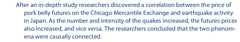
The argument is clearly weak. Because it is virtually inconceivable that either phenomenon could cause a change in the other, or that changes in both could have a common cause, it is most likely that the correlation is purely coincidental.
The method of concomitant variation is useful when it is impossible for a condition to be either wholly present or wholly absent, as was required for the use of the first three of Mill’s methods. Many conditions are of this sort—for example, the temperature of the ocean, the price of gold, the incidence of crime, the size of a mountain glacier, a person’s cholesterol level, and so on. If some kind of correlation can be detected between variations in conditions such as these, the method of concomitant variation asserts that the two are causally connected. The method has been used successfully in the past to help establish the existence of causal connections between smoking and lung cancer, nuclear radiation and leukemia, and alcohol consumption and cirrhosis of the liver.
10.3 Mill’s Methods and Science
Mill’s methods closely resemble certain scientific methods that are intended to establish causal connections and correlations. For example, the method of difference is virtually identical to the method of controlled experiment employed in such fields as biology, pharmacology, and psychology. A controlled experiment is one that involves two groups of subjects, an experimental group and a control group. The experimental group includes the subjects that receive a certain treatment, and the control group includes the subjects that do not receive the treatment but are otherwise subjected to the same conditions as the experimental group.
The simplest type of controlled experiment involves an experimental group and a control group each consisting of just one member. Example:
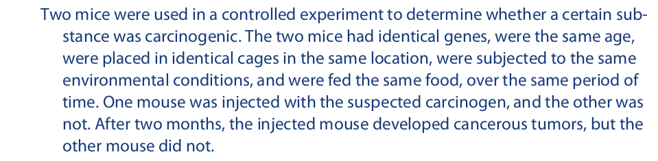
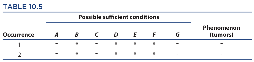
To summarize the results of this experiment we can construct a table just like the one for the method of difference. If we let occurrence 1 represent the injected mouse and occurrence 2 the mouse that was not injected, and let A through F represent the conditions common to the two mice (genes, age, cage, etc.) and G represent the injection, we have Table 10.5. Using the rule that a condition is not sufficient if it is present when the phenomenon is absent, occurrence 2 eliminates A through F, leaving G (the suspected carcinogen) as the cause of the phenomenon.
The principal drawback of this experiment is that the suspected carcinogen was given to only one mouse. As a result, the experiment offers relatively weak evidence that any mouse injected with this substance would develop tumors. Perhaps the injected mouse had some hidden defect that would have caused tumors even without the injection. Scientists address this problem by increasing the size of the experimental group and the control group. Thus, suppose the same experiment were performed on one hundred mice, of which fifty were injected and fifty were not. Suppose that after two months all fifty injected mice developed tumors and none of the control subjects did. Such a result would constitute much stronger evidence that the injected substance was carcinogenic.
This expanded experiment can be considered to be a case of multiple uses of Mill’s method of difference. Since the method of difference always involves just two occurrences, mouse #1 could be matched with mouse #51 for one use of the method, mouse #2 with mouse #52 for a second use of the method, and so on. Although this expanded experiment might look like a case of the joint method, it is not (at least not a successful one). Any successful application of the joint method includes occurrences in which certain conditions are absent when the phenomenon is present. Those conditions are then eliminated as possible necessary conditions. The expanded experiment with the mice includes no such occurrences.
This fact points up an important difference between Mill’s joint method and his method of difference. The purpose of the method of difference is to determine whether a preselected condition is the cause of a phenomenon. This preselected condition is present in one of the two occurrences and absent from the other. On the other hand, the purpose of the joint method is to determine which condition, among a selected class of conditions, is a cause of a phenomenon. The joint method applies rules for sufficient conditions and necessary conditions to (one hopes) reduce the class of conditions to just one.
Returning to the expanded experiment with the mice, let us suppose that only forty of the mice in the experimental group developed tumors, and none of those in the control group did. From Mill’s standpoint, this would be equivalent to forty uses of the method of difference yielding positive results and ten yielding negative results. On the basis of such an outcome, the experimenter might conclude that the likelihood of the suspected carcinogen producing tumors in mice was 80 percent (40 ÷ 50).
Controlled experiments such as the one involving a hundred mice are often conducted on humans, but with humans it is never possible to control the circumstances to the degree that it is with mice. Humans cannot be put in cages or fed exactly the same food for any length of time, are not genetically identical to other humans, and so forth. Also, humans react to their environment in ways that cannot be anticipated or controlled. To correct this deficiency, statistical methods are applied to the results to enable the drawing of a conclusion.
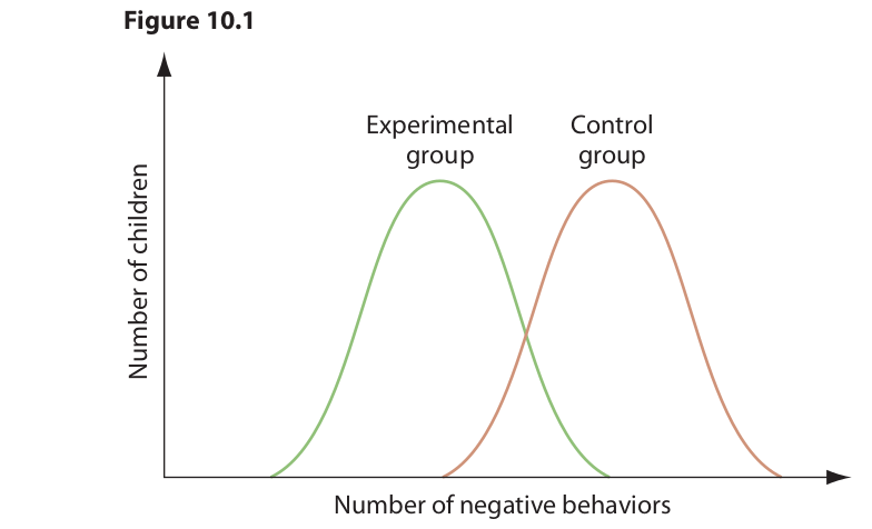
For example, an experiment could be conducted to test the effectiveness of some new drug on children with attention deficit/hyperactivity disorder (ADHD). Fifty children with ADHD could be selected, with twenty-five being placed at random in the experimental group and twenty-five in the control group. The children in the experimental group would be given the drug, probably in a classroom situation, and the children in the control group would be given a placebo (sugar pill). This could be done on a “double blind” basis, so that neither the children nor the people conducting the experiment would know in advance who was getting the drug. The objective is to control the conditions as much as possible. Then the negative behavior of each of the fifty children would be recorded over a period, say, of an hour. Each time a child was out of his or her seat, disturbed others, fidgeted, failed to follow instructions, and so forth, the incident would be noted.
The results of such an experiment would be expected to follow what is called a normal probability distribution (bell-shaped curve). (Further discussion of normal probability distribution is presented in Chapter 12.) One curve would represent the experimental group, another curve the control group. Assuming the drug is effective, the two curves would be displaced from one another, but they would probably overlap in part, as indicated in Figure 10.1. This means that certain children in the experimental group exhibited more negative behaviors than certain children in the control group, but most of the children in the experimental group exhibited fewer negative behaviors than most of the children in the control group. Then statistical methods would be applied to the two curves to determine the effectiveness of the drug. Such an experiment is similar to Mill’s method of difference except that instead of the phenomenon (negative behavior) being wholly present in some occurrences, it is present in varying degrees. In this sense, the experiment resembles the method of concomitant variation.
In some kinds of scientific research on humans, controlling the circumstances to any significant degree is nearly impossible. Such research includes investigations that cover a long period or investigations in which the health of the subjects is at issue and legal or moral restrictions come into play. Example:
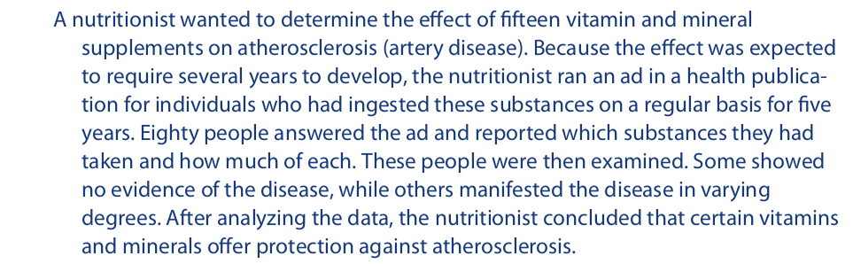
The procedure followed by the nutritionist is very similar to Mill’s joint method of agreement and difference. The objective is to identify a cause among a preselected class of possible conditions, some of which are accompanied by the phenomenon (atherosclerosis), and some of which are not. The major difference between the nutritionist’s procedure and Mill’s joint method is that the nutritionist took account of varying degrees in which the conditions and the phenomenon were present in the eighty occurrences. In this sense, again, the nutritionist’s procedure was similar to Mill’s method of concomitant variation. However, the nutritionist may also have taken into account various combinations of conditions, a consideration that lies beyond the power of the joint method by itself.
The procedure illustrated in this example is not an experiment but a study. More precisely, it is a retrospective study because it examines subjects who have already fulfilled the requirements of the examination—as opposed to a prospective study, where the subjects are expected to fulfill the requirements in the future. For a prospective study, the nutritionist could select a group of subjects and follow their future vitamin and mineral intake for five years. Such a study, however, would be more costly, and if the nutritionist instructed the subjects to ingest certain vitamins and minerals and avoid others, the study could involve legal or moral implications.
Another kind of study found widely in the social sciences uses what is called the correlational method, which closely replicates Mill’s method of concomitant variation. Example:
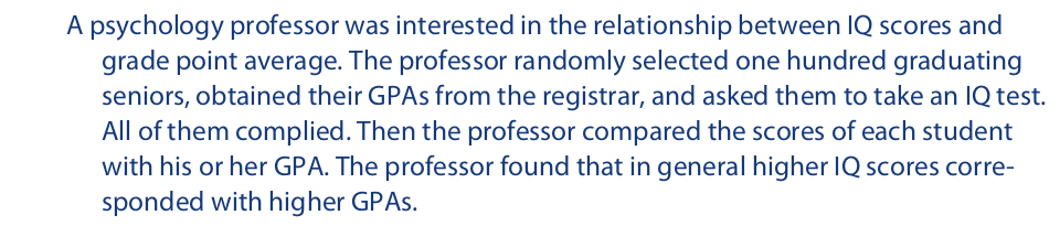
The results of this study indicate a positive correlation between IQ score and GPA. If the study showed that students with higher IQs had, in general, lower GPAs, this would indicate a negative correlation. Once a study of this sort is done, the next step is to compute the correlation coefficient, which is a number between +1.00 and –1.00 that expresses the degree of correlation. If it turned out that the student with the highest IQ score also had the highest GPA, the student with the next highest IQ score had proportionately the next highest GPA, and so on, so that the IQ-GPA graph was a straight line, then the correlation coefficient would be +1.00. This would reflect a perfect positive correlation.
On the other hand, if it turned out that the student with the highest IQ score had the lowest GPA, the student with the next highest IQ score had proportionately the next lowest GPA, and so on, so that, once again, the IQ-GPA graph was a straight line, then the correlation coefficient would be −1.00. This would reflect a perfect negative correlation. A correlation coefficient of 0.00 would mean that no correlation exists, which would be the case if the IQ scores corresponded randomly with the GPAs. A correlation coefficient of, say, +0.60 would mean that in general higher IQ scores corresponded positively with higher GPAs.
The outcome of this study can also be indicated graphically, with IQ score representing one coordinate on a graph, and GPA the other coordinate. The result for each student would then correspond to a point on the graph, such as the one in Figure 10.2. The graph of all the points is called a scatter diagram. A line that “best fits” the data can then be drawn through the scatter diagram. This line is called the regression line, and it can be used to produce a linear equation, y = bx + a, that describes the approximate relation between IQ score (x) and GPA (y). This equation can then be used to predict future GPAs. For example, suppose that an entering freshman student has an IQ of 116. This student’s future GPA could be predicted to be approximately 116b + a.

Hundreds of studies such as this one have been conducted to detect correlations between such factors as TV violence and aggression in children, self-esteem and intelligence, motivation and learning time, exposure to classical music and retention ability, and marijuana use and memory. However, such studies often fall short of establishing a causal connection between the two factors. For example, a positive correlation between exposure to TV violence and aggression in children does not necessarily mean that exposure to TV violence causes aggression. It might be the case that children who tend to be violent are naturally attracted to violent TV shows. Or perhaps a third factor is the cause of both. But a positive correlation can at least suggest a causal connection.
Once a correlation is established, a controlled experiment can often be designed that will identify a causal connection. For example, in the case of TV violence, a group of children could be randomly divided into an experimental group and a control group. The experimental group could then be exposed to violent TV shows for a certain period, and the control group would be exposed to nonviolent shows for the same period. Later, the behavior of the children in both groups could be observed, with every act of aggression noted. If the experimental group displayed more acts of aggression than the control group, the conclusion might be drawn that TV violence causes aggression.
Experimental procedures resembling Mill’s method of concomitant variation have also been used in the physical sciences to identify causal connections. For example, in the early part of the nineteenth century, Hans Christian Oerstead noticed that a wire carrying a current of electricity could deflect a nearby compass needle. As the current was increased, the amount of deflection increased, and as the current was decreased, the amount of deflection decreased. Also, if the current were reversed, the deflection would be reversed. Oerstead concluded that a current of electricity flowing through a wire causes a magnetic field to be produced around the wire.
Other applications of the method of concomitant variation have been used not so much to detect the existence of a causal connection (which may have already been known) as to determine the precise nature of a causal law. For example, in the latter part of the sixteenth century Galileo performed experiments involving spheres rolling down inclined planes. As the plane was incrementally lifted upward, the sphere covered greater and greater distances in a unit of time. Recognizing that the downward force on the sphere is proportional to the pitch of the plane, Galileo derived the law that the acceleration imparted to a body is directly proportional to the force acting on it. Galileo also noticed that whatever the angle of the plane, the distance covered by the ball increased exponentially with the time in which it was allowed to roll. For example, if the time was doubled, the distance was quadrupled. From this correlation he derived the law that the distance traveled by a falling body is proportional to the square of the time that it falls.
In the seventeenth century, Robert Boyle conducted experiments involving the pressure and volume of gases. Boyle constructed an apparatus that allowed him to compute the volume of a gas as he varied the pressure. He noted that as the pressure increased, the volume decreased, and as the pressure decreased, the volume increased. From this correlation he derived the law that the volume of a gas is inversely proportional to its pressure. A century later, Jacques Alexandre Charles observed a correlation between the temperature of a gas and its volume. As the temperature increased, the volume increased, and vice versa. This correlation provided the basis for Charles’s law for gases.
Detecting correlations has also been important in astronomy. Early in the twentieth century, Henrietta Swan Leavitt recognized a correlation between the average brightness of certain variable stars, called Cepheids (pronounced sef⬘-ee-ids), and their periods of variation. Cepheids fluctuate in brightness over periods ranging from a day to several months, and Leavitt discovered that longer periods correspond with greater average brightness, and shorter periods with lesser average brightness. Once the distance of a few nearby Cepheids was determined, the distance of any Cepheid could then be computed from its average brightness and its period of variation. This correlation provided the first method available to astronomers for measuring the distance between our planet and galaxies other than our own.


 浙公网安备 33010602011771号