深度学习的始祖框架，grandfather级别的框架 —— Theano —— 示例代码学习（1）

示例代码1：

import theano
from theano import tensor

x = tensor.vector("x")
y = tensor.vector("y")
w = tensor.vector("w")
z = tensor.vector("z")

z = x+y+w

f = theano.function([x, theano.In(y, value=[1,1,1]), theano.In(w,value=[2,2,2], name='weights')], z)

# 不使用默认值
print( f([1,2,3], [2,3,4], [3,4,5]) )

# 使用默认值
print( f([1,2,3], [2,3,4]) )
print( f([1,2,3], weights=[2,3,4]) )
print( type(f([1,2,3], weights=[2,3,4])) )

运行结果：

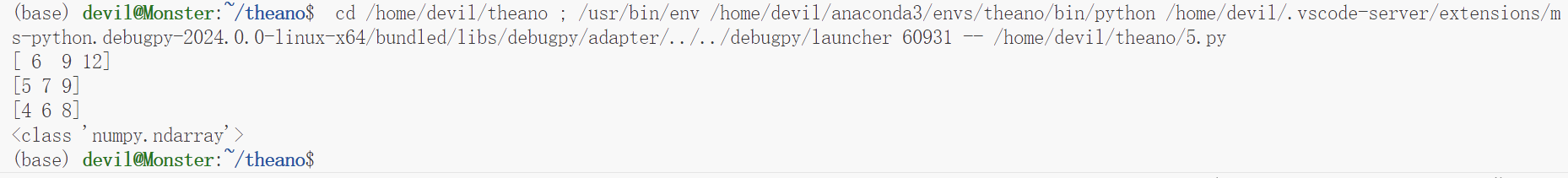
示例代码2：（与示例代码1不同的地方在于设置变量数据类型为int而不是默认的double，即vector和ivector的区别）

import theano
from theano import tensor

x = tensor.ivector("x")
y = tensor.ivector("y")
w = tensor.ivector("w")
z = tensor.ivector("z")

z = x+y+w

f = theano.function([x, theano.In(y, value=[1,1,1]), theano.In(w,value=[2,2,2], name='weights')], z)

# 不使用默认值
print( f([1,2,3], [2,3,4], [3,4,5]) )

# 使用默认值
print( f([1,2,3], [2,3,4]) )
print( f([1,2,3], weights=[2,3,4]) )
print( type(f([1,2,3], weights=[2,3,4])) )

运行结果：

代码3：（加1操作，并复制给变量实现update的目的）

import theano
from theano import tensor


state = theano.shared(0)

inc = tensor.iscalar('inc')

# accumulator = theano.function([inc], [], updates=[(state, state+inc), ])
accumulator = theano.function([inc], state, updates=[(state, state+inc), ])


print(state.get_value())

print(accumulator(1))

print(state.get_value())

运行结果：

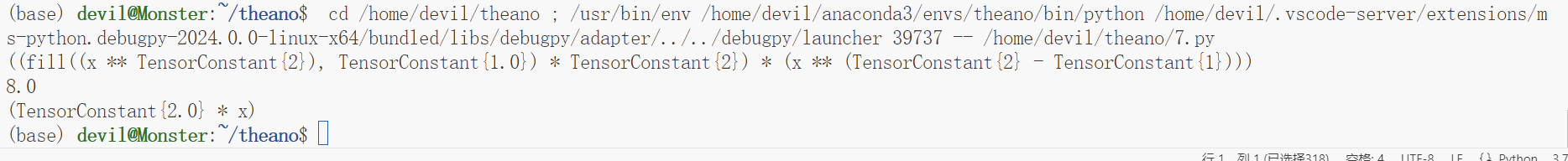
代码4：（求导操作）

import theano

import theano.tensor as tensor

x = tensor.dscalar('x')

y = x ** 2 # 定义函数y=x^2

gy = tensor.grad(y, x) # 导函数的表达式

f = theano.function([x], gy) # 将导函数编译成Theano函数


print( theano.pp(gy) )  # 打印优化之前的导函数表达式


print( f(4) )  # 带入数据计算x=4时的导数值


print( theano.pp(f.maker.fgraph.outputs[0]) )  # 打印编译优化后的导函数表达式

运行结果：

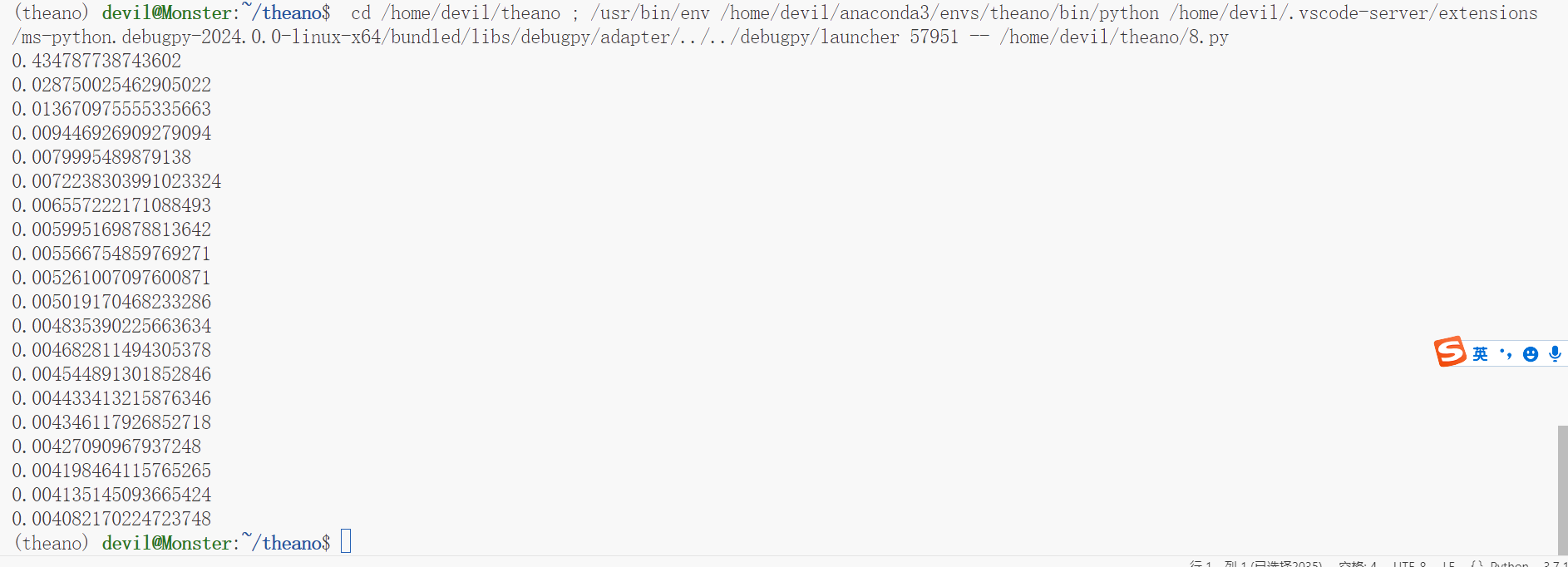
代码5：（神经网络实现2层MLP预测训练）

import theano

import theano.tensor as tensor

import numpy as np

import matplotlib.pyplot as plt  #引入了matplotlib这个工具包, 用来实现绘图及数据可视化。


"""
定义层结构
接下来我们声明我们的Layer类
对于神经网络的每个Layer, 它需要具备输入来源input, 输入神经元维度in_size, 输出神经元纬度out_size,
和我们之前设计的神经元的激活函数activation_function, 默认为None。
"""

class Layer(object):
    def __init__(self, inputs, in_size, out_size, activation_function=None):
        self.W = theano.shared(np.random.normal(0, 1, (in_size, out_size)))
        self.b = theano.shared(np.zeros((out_size, )) + 0.1)
        self.Wx_plus_b = tensor.dot(inputs, self.W) + self.b
        self.activation_function = activation_function

        if activation_function is None:
            self.outputs = self.Wx_plus_b
        else:
            self.outputs = self.activation_function(self.Wx_plus_b)

"""
伪造数据
接下来，我们首先人工生成一个简单的带有白噪声的一维数据 y = x^2 - 0.5 + noise。
"""
# Make up some fake data
x_data = np.linspace(-1, 1, 300)[:, np.newaxis]
noise = np.random.normal(0, 0.05, x_data.shape)
y_data = np.square(x_data) - 0.5 + noise    # y = x^2 - 0.5 + wihtenoise

# show the fake data
plt.scatter(x_data, y_data)
plt.show()


# determine the inputs dtype
x = tensor.dmatrix("x")
y = tensor.dmatrix("y")

# determine the inputs dtype
# add layers
l1 = Layer(x, 1, 10, tensor.nnet.relu)
l2 = Layer(l1.outputs, 10, 1, None)

# compute the cost
cost = tensor.mean(tensor.square(l2.outputs - y))

# compute the gradients
gW1, gb1, gW2, gb2 = tensor.grad(cost, [l1.W, l1.b, l2.W, l2.b])

# apply gradient descent
learning_rate = 0.05
train = theano.function(inputs=[x, y], outputs=cost, \
                        updates=[(l1.W, l1.W - learning_rate * gW1), \
                                (l1.b, l1.b - learning_rate * gb1), \
                                (l2.W, l2.W - learning_rate * gW2), \
                                (l2.b, l2.b - learning_rate * gb2)])

# prediction
predict = theano.function(inputs=[x], outputs=l2.outputs)

for i in range(1000):
    # training
    err = train(x_data, y_data)
    if i % 50 == 0:
        print(err)

运行结果：

参考：

https://www.jianshu.com/p/1f55c446ce3a