收益率曲线交易的分析框架

目录

• A Framework for Analyzing Yield Curve Trades
  • INTRODUCTION
  • FORWARD RATES AND THEIR DETERMINANTS
    • How Do the Main Determinants Influence the Yield Curve Shape?
    • Decomposing Forward Rates Into Their Main Determinants
  • DECOMPOSING EXPECTED RETURNS OF BOND POSITIONS
    • Five Alternative Expected Return Measures
    • Link to Scenario Analysis
  • APPENDIX A. DECOMPOSING THE FORWARD RATE STRUCTURE INTO ITS MAIN DETERMINANTS
  • APPENDIX B. RELATING VARIOUS STATEMENTS ABOUT FORWARD RATES TO EACH OTHER

著：Antti Ilmanen 译：徐瑞龙

更新：修正原文中的一处错误

A Framework for Analyzing Yield Curve Trades

收益率曲线交易的分析框架

INTRODUCTION

引言

In Part 1 of this series, Overview of Forward Rate Analysis, we argued that the shape of the yield curve depends on three factors: the market's rate expectations; the required bond risk premia; and the convexity bias. After examining these determinants in detail in Parts 2-5, we now return to the "big picture" to show how we can decompose the forward rate curve into these three determinants. Even though we cannot directly observe these determinants, the decomposition can clarify our thinking about the yield curve.

在本系列的第1部分（《远期收益率分析概述》）中，我们认为收益率曲线的形状取决于三个因素：市场收益率预期、债券风险溢价和凸度偏差。在第2-5部分详细研究了这些决定因素后，我们现在回到“大局”上，显示如何将远期收益率曲线分解为这三个决定因素。即使我们不能直接观察这些决定因素，分解可以理清我们对收益率曲线的思考。

Our analysis also produces direct applications —— it provides a systematic framework for relative value analysis of noncallable government bonds. Analogous to the decomposition of forward rates, the total expected return of any government bond position can be viewed as the sum of a few simple building blocks: (1) the yield income; (2) the rolldown return; (3) the value of convexity; and (4) the duration impact of the rate view. A fifth term, the financing advantage, should be added for bonds that trade "special" in the repo market.

我们的分析也产生了直接的应用，它提供了一个系统的框架，用于非可赎回政府债券的相对价值分析。类似于远期收益率的分解，任何政府债券头寸的总预期回报可以被看作是几个简单因素的总和：（1）收益率回报；（2）下滑回报；（3）凸度价值和（4）久期影响。还有第五个因素——融资优势，这是在回购市场上被“特殊”对待的债券所具有的。

The following observations motivate this decomposition. A bond's near-term expected return is a sum of its horizon return given an unchanged yield curve and its expected return from expected changes in the yield curve. The first item, the horizon return, is also called the rolling yield because it is a sum of the bond's yield income and the rolldown return (the capital gain that the bond earns because its yield declines as its maturity shortens and it "rolls down" an upward-sloping yield curve). The second item, the expected return from expected changes in the yield curve, can be approximated by duration and convexity effects. The duration impact is zero if the yield curve is expected to remain unchanged, but it may be the main source of expected return if the rate predictions are based on a subjective market view or on a quantitative forecasting model. The value of convexity is always positive and depends on the bonds convexity and on the perceived level of yield volatility.

以下观察结果启发了这种分解。债券的近期预期回报是收益率曲线不变情况下的持有期回报及收益率曲线预期变化带来的预期回报的和。第一个部分，即持有期回报，也被称为滚动收益率，因为它是债券收益率和下滑回报（在向上倾斜的收益率曲线上收益率随着其期限的缩短而下降，收益率在曲线上“下滑”而使得债券赚取的资本回报）的总和。第二个部分，收益率曲线预期变化带来的预期回报，可以由久期和凸度来近似。如果预期收益率曲线保持不变，则久期影响为零，但久期影响可能是预期回报的主要来源，如果收益率预测基于主观的市场观点或量化预测模型。凸度价值总是为正的，并取决于债券的凸度和收益率波动率的水平。

We argue that both prospective and historical relative value analysis should focus on near-term expected return differentials across bond positions instead of on yield spreads. The former measures take into account all sources of expected return. Moreover, they provide a consistent framework for evaluating all types of government bond positions. We also show, with practical examples, how various expected return measures are computed and how our framework for relative value analysis is related to the better-known scenario analysis.

我们认为，前瞻性和历史性的相对价值分析都应该关注债券头寸的近期预期回报差异，而不是利差。前者考虑到所有的预期回报来源。此外，近期预期回报差异为评估各类政府债券头寸提供了一个一致的框架。我们还通过实际的例子，展示了各种预期回报的计算方法，以及我们的相对价值分析框架如何与更为众所周知的情景分析相关。

FORWARD RATES AND THEIR DETERMINANTS

远期收益率及其决定因素

How Do the Main Determinants Influence the Yield Curve Shape?

主要决定因素如何影响收益率曲线形状

We first describe how the market's rate expectations, the required bond risk premia^[1], and the convexity bias influence the term structure of spot and forward rates. The market's expectations regarding the future interest rate behavior are probably the most important influences on today's term structure. Expectations for parallel increases in yields tend to make today's term structure linearly upward sloping, and expectations for falling yields tend to make today's term structure inverted. Expectations for future curve flattening induce today's spot and forward rate curves to be concave (functions of maturity), and expectations for future curve steepening induce today's spot and forward rate curves to be convex.^[2] These are the facts, but what is the intuition behind these relationships?

我们首先描述市场的收益率预期、债券风险溢价以及凸度偏差如何影响即期和远期收益率的期限结构。市场对未来收益率行为的预期可能是对当下期限结构最重要的影响因素。收益率水平上升的预期倾向于使当下的期限结构呈线性向上倾斜，对收益率下降的预期倾向于使当下的期限结构倒挂。对未来曲线变平的预期会导致当下的即期和远期收益率曲线为上凸的（作为期限的函数），对未来曲线变陡的预期会导致当下的即期和远期收益率曲线是下凸的。这些是事实，但这些关系背后的直觉是什么？

The traditional intuition is based on the pure expectations hypothesis. In the absence of risk premia and convexity bias, a long rate is a weighted average of the expected short rates over the life of the long bond. If the short rates are expected to rise, the expected average future short rate (that is, the long rate) is higher than the current short rate, making today's term structure upward sloping. A similar logic explains why expectations of falling rates make today's term structure inverted. However, this logic gives few insights about the relation between the market's expectations regarding future curve reshaping and the curvature of today's term structure.

传统上，直觉基于完全预期假说。在没有风险溢价和凸度偏差的情况下，长期收益率是长期债券存续期内预期的短期收益率的加权平均值。如果预期短期收益率上涨，预期的未来平均短期收益率（即长期收益率）高于目前的短期收益率，使得当下的期限结构向上倾斜。类似的逻辑解释了为什么对预期收益率下降使当下的期限结构倒挂。然而，这个逻辑对于解释市场对未来曲线形变的预期与当下期限结构的曲率之间的关系几乎没有帮助。

Another perspective to the pure expectations hypothesis may provide a better intuition. The absence of risk premia means that all bonds, independent of maturity, have the same near-term expected return. Recall that a bond's holding-period return equals the sum of the initial yield and the capital gains/losses that yield changes cause. Therefore, if all bonds are to have the same expected return, initial yield differentials across bonds must offset any expected capital gains/losses. Similarly, each bond portfolio with expected capital gains must have a yield disadvantage relative to the riskless asset. If investors expect the long bonds to gain value because of a decline in interest rates, they accept a lower initial yield for long bonds than for short bonds, making today's spot and forward rate curves inverted. Conversely, if investors expect the long bonds to lose value because of an increase in interest rates, they demand a higher initial yield for long bonds than for short bonds, making today's spot and forward rate curves upward sloping. Similarly, if investors expect the curve-flattening positions to earn capital gains because of future curve flattening, they accept a lower initial yield for these positions. In such a case, barbells would have lower yields than duration-matched bullets (to equate their near-term expected returns), making today's spot and forward rate curves concave. A converse logic links the market's curve-steepening expectations to convex spot and forward rate curves.

完全预期假说的另一个观点可能会提供更好的直觉。没有风险溢价意味着，无论期限多少，所有债券具有相同的近期预期回报。回想一下，债券的持有期回报等于初始收益率和收益率变化引起的资本损益的总和。因此，如果所有债券都具有相同的预期回报，则债券之间的初始收益率差异必须抵消任何预期的资本损益。同样，每个具有预期资本回报的债券组合都必须相对于无风险资产的存在收益率上的劣势。如果投资者预期长期债券由于收益率下降而获得价值，则他们接受长期债券的初始收益率低于短期债券，使得当下的即期和远期收益率曲线倒挂。相反，如果投资者预期长期债券由于收益率上升而失去价值，则他们要求长期债券的初始收益率高于短期债券，使得当下的即期和远期收益率曲线向上倾斜。同样，如果投资者预期做平曲线的头寸由于未来曲线变平而获得资本回报，他们接受这些头寸的初始收益率较低。在这种情况下，杠铃组合的收益率将低于久期匹配的子弹组合（使得近期预期回报相等），使当下的即期和远期收益率曲线变得上凸。相反的逻辑将市场的曲线变陡的预期与即期和远期收益率曲线下凸联系起来。

The above analysis presumes that all bond positions have the same near-term expected returns. In reality, investors require higher returns for holding long bonds than short bonds. Many models that acknowledge bond risk premia assume that they increase linearly with duration (or with return volatility) and that they are constant over time. Parts 3 and 4 of this series showed that empirical evidence contradicts both assumptions. Historical average returns increase substantially with duration at the front end of the curve but only marginally after the two-year duration. Thus, the bond risk premia make the term structure upward-sloping and concave, on average. Moreover, it is possible to forecast when the required bond risk premia are abnormally high or low. Thus, the time-variation in the bond risk premia can cause significant variation in the shape of the term structure.

上述分析假设所有债券头寸都具有相同的近期预期回报。实际上，投资者要求持有长期债券的回报比短期债券要高。许多模型接受债券风险溢价的存在，并且假设它们随久期（或回报波动率）线性增加以及随时间恒定。本系列的第3和第4部分显示，实证证据与两种假设相矛盾。历史平均回报在曲线前端关于久期大幅度增长，但在两年久期后只是略有增长。因此，债券风险溢价使得期限结构向上倾斜并上凸。此外，有可能预测债券风险溢价何时异常高或低。因此，债券风险溢价的时变性可能导致期限结构形状的显着变化。

Convexity bias refers to the impact that the nonlinearity of a bond's price-yield curve has on the shape of the term structure. This impact is very small at the front end but can be quite significant at very long durations. A positively convex price-yield curve has the property that a given yield decline raises the bond price more than a yield increase of equal magnitude reduces it. All else equal, this property makes a high-convexity bond more valuable than a low-convexity bond, especially if the volatility is high. It follows that investors tend to accept a lower initial yield for a more convex bond because they have the prospect of enhancing their returns as a result of convexity. Because a long bond exhibits much greater convexity than a short bond, it can have a lower yield and yet, offer the same near-term expected return. Thus, in the absence of bond risk premia, the convexity bias would make the term structure inverted. In the presence of positive bond risk premia, the convexity bias tends to make the term structure humped —— because the negative effect of convexity bias overtakes the positive effect of bond risk premia only at long durations. An increase in the interest rate volatility makes the bias stronger and, thus, tends to make the term structure more humped.

凸度偏差是指债券的价格-收益率曲线的非线性对期限结构的影响。这种影响在短久期端非常小，但在长久期端可能会相当显着。一个正凸度的价格-收益率曲线使得收益率下降带来的债券价格提高程度大于收益率上升带来的债券价格降低程度。其他条件都相同的情况下，这种特性使得高凸度债券比低凸度债券更有价值，特别是波动率高的情况下。因此，对于凸度更大的债券，投资者倾向于接受较低的初始收益率，因为凸度有增加回报的效果。在近期预期回报相同的前提下，由于长期债券比短期债券具有更大的凸度，所以它的收益率可能会较低。因此，在没有债券风险溢价的情况下，凸度偏差将使期限结构倒挂。在存在正的债券风险溢价的情况下，凸度偏差倾向于使期限结构隆起——由于在长久期端凸度偏差的负面影响超过债券风险溢价的正面影响。收益率波动性的增加使得凸度偏差更大，因此趋向于使期限结构更加隆起。

The three determinants influence the shape of the term structure simultaneously, making it difficult to distinguish their individual effects. One central theme in this series has been that the shape of the term structure does not only reflect the market's rate expectations. Forward rates are good measures of the market's rate expectations only if the bond risk premia and the convexity bias can be ignored. This is hardly the case, even though a large portion of the short-term variation in the shape of the curve probably reflects the market's changing expectations about the future level and shape of the curve. The steepness of the curve on a given day depends mainly on the market's view regarding the rate direction, but in the long run, the impact of positive and negative rate expectations largely washes out. Therefore, the average upward slope of the yield curve is mainly attributable to positive bond risk premia. The curvature of the term structure may reflect all three components. On a given day, the spot rate curve is especially concave (humped) if market participants have strong expectations of future curve flattening or of high future volatility. In the long run, the reshaping expectations should wash out, and the average concave shape of the term structure reflects the concavity of the risk premium curve and the convexity bias.

三个决定因素同时影响期限结构的形状，使得难以区分其各自的作用。这个系列的一个中心主题是，期限结构的形状不仅仅反映了市场的收益率预期。只有债券风险溢价和凸度偏差可以忽略，远期收益率才是市场收益率预期的良好指标。事实并非如此，尽管很大程度上曲线形状的短期变化反映了市场对曲线未来水平和形状的变化预期。曲线在某一天的陡峭程度主要取决于市场对收益率方向的看法，但从长远来看，正负收益率预期的影响大部分被淘汰。因此，平均来看向上倾斜的收益率曲线主要归咎于债券风险溢价。期限结构的曲率可能反映所有三个成分。在某一天，如果市场参与者对未来曲线变平或未来波动率变大有强烈的预期，则即期收益率曲线尤其是上凸的。从长远来看，曲线形变的预期会被淘汰，而平均来看期限结构的上凸形状反映了风险溢价曲线的凸度和凸度偏差。

Decomposing Forward Rates Into Their Main Determinants

分解远期收益率

Conceptually, each one-period forward rate can be decomposed to three parts: the impact of rate expectations; the bond risk premium; and the convexity bias. So far, this statement is just an assertion. In this subsection, we show intuitively why this relationship holds between the forward rates and their three determinants. We provide a more formal derivation in Appendix A (where we take into account the fact that the analysis is not instantaneous but yield changes occur over a discrete horizon, during which invested capital grows). In Appendix B, we tie some loose strings together by summarizing various statements about the forward rates and by clarifying the relations between these statements.

从概念上讲，每一期远期收益率都可以分解为三个部分：收益率预期的影响、债券风险溢价和凸度偏差。到目前为止，这个说法只是一个断言。在本小节中，我们直观地展示为什么远期收益率与其三个决定因素之间存在这种关系。我们在附录A中提供更正式的推导（在那里我们考虑到分析不是即时的，而是在收益率发生变化的一段时期）。在附录B中，我们通过总结关于远期收益率的各种陈述以及理清这些陈述之间的关系，将一些松散的结论串联在一起。

Figure 1 shows how the yield change of an n-year zero-coupon bond over one period (dashed arrow) can be split to the rolldown yield change and the one-period change in an n-1 year constant-maturity spot rate \(s_{n-1}\) (\(\Delta s_{n-1} = s^*_{n-1} - s_{n-1}\)) (two solid arrows).^[3] A zero-coupon bond's price can be split in a similar way (see Appendix A). Thus, an n-year zero's holding-period return over the next period \(h_n\) is:

图1显示了在一个时期n年期零息债券的收益率变化（虚线箭头）如何可以分解为滚动收益率的变化和n-1年期即期收益率\(s_{n-1}\)的变化（\(\Delta s_{n-1} = s^*_{n-1} - s_{n-1}\)，两个实线箭头）。零息债券的价格可以以类似的方式分解（见附录A）。因此，n年期零息债券的一（年）期持有期回报\(h_n\)为：

\[\begin{aligned} h_n &= \text{return if curve is unchanged} &+& [\text{return from the curve changes}] \\ &= \text{rolling yield} &+& [\text{percentage price change (at horizon)}] \\ &\approx \text{(one-period) forward rate} &+& [-\text{duration} * (\Delta s_{n-1}) + 0.5*\text{convexity} * (\Delta s_{n-1})^2] \end{aligned} \tag{1} \]

Figure 1 Splitting a Zero-Coupon Bond's One-Period Yield Change Into Two Parts

Equation (1) is based on the following relations. First, a bond's one-period horizon return given an unchanged yield curve is called the rolling yield. A zero-coupon bond's rolling yield equals the one-period forward rate (\(f_{n-1,n}\)). For example, if the four-year (five-year) constant-maturity rate remains unchanged at 9.5% (10%) over the next year, a five-year zero bought today at 10% can be sold next year at 9.5%, as a four-year zero; then the bonds horizon return is \(1.10^5 / 1.095^4 - 1 = 12.02\%\), which is the one-year forward rate between four- and five-year maturities (see Equation (12) in Appendix B). The second source of a zero's holding-period return, the price change caused by the yield curve shift, is approximated very well by duration and convexity effects for all but extremely large yield curve shifts.

等式（1）基于以下关系。首先，给定不变收益率曲线的债券一（年）期持有期回报称为滚动收益率。零息债券的滚动收益率等于一（年）期远期收益率（\(f_{n-1,n}\)）。例如，如果四年（五年）收益率在未来一年保持不变，为9.5%（10%），那么今年以10%的收益率购买的五年期零息债券下一年将以9.5%的收益率出售，那么债券持有期回报为12.02%，即四年到五年期间的一年期远期收益率（见附录B中的等式（12））。零息债券回报的第二个来源，即收益率曲线变动引起的价格变动，能用久期和凸度很好的近似，除非收益率曲线发生非常大的变化。

It is more interesting to relate the forward rates to expected returns and expected rate changes than to the realized ones. We take expectations of both sides of Equation (1), split the bond's expected holding-period return into the short rate and the bond risk premium, and recall that \(E(\Delta s_{n-1})^2 \approx (Vol(\Delta s_{n-1}))^2\). Then we can rearrange the equation to express the one-period forward rate as a sum of the other terms:

相对于已实现收益率，将远期收益率与预期回报和预期收益率变动相联系将会更有意义。我们对等式（1）的两边取期望，将债券的预期持有期回报分为短期收益率和债券风险溢价两部分，并回顾\(E(\Delta s_{n-1})^2 \approx (Vol(\Delta s_{n-1}))^2\)。然后，我们可以重新排列等式，将远期收益率作为其他项的和：

\[\text{Forward rate} \approx \text{short rate} + \text{duration} * E(\Delta s_{n-1}) + \text{bond risk premium} + \text{convexity bias}, \tag{2} \]

where bond risk premium = \(E(h_n - s_1)\) and convexity bias \(\approx -0.5 * \text{convexity}*(Vol(\Delta s_{n-1}))^2\).

其中债券风险溢价=\(E(h_n - s_1)\)，凸度偏差\(\approx -0.5 * \text{convexity}*(Vol(\Delta s_{n-1}))^2\)。

If we move the short rate to the left-hand side of the equation, we decompose the "forward-spot premium" (\(f_{n-1, n} - s_1\)) into a rate expectation term, a risk premium term and a convexity term (see Equation (11) in Appendix A). We interpret the expectations in Equation (2) as the market's rate and volatility expectations and as the expected risk premium that the market requires for holding long-term bonds. The market's expectations are weighted averages of individual market participants' expectations.

如果我们将短期收益率移动到等式的左边，我们将“远期-即期溢价”（\(f_{n-1, n} - s_1\)）分解为预期收益率、风险溢价和凸度项（见附录A中的等式（11））。我们将等式（2）中的预期值视为市场收益率和波动率的预期值，以及持有长期债券所需的预期风险溢价。市场预期是个体市场参与者预期的加权平均值。

Some readers may wonder why our analysis deals with forward rates and not with the more familiar par and spot rates. The reason is the simplicity of the one-period forward rates. A one-period forward rate is the most basic unit in term structure analysis, the discount rate of one cash flow over one period. A spot rate is the average discount rate of one cash flow over many periods, whereas a par rate is the average discount rate of many cash flows —— those of a par bond —— over many periods. All the averaging makes the decomposition messier for the spot rates and the par rates than it is for the one-period forward rate in Equation (2). However, because the spot and the par rates are complex averages of the one-period forward rates, they too can be conceptually decomposed into the three main determinants.

一些读者可能会想知道为什么我们的分析涉及远期收益率，而不是更熟悉的到期和即期收益率。原因是一年期远期收益率的简单性。一年期远期收益率是期限结构分析中最基本的单位，即一年期现金流贴现率。即期收益率是多期现金流的平均贴现率，而到期收益率是许多多期现金流的平均贴现率。所有的平均化使得对于即期收益率和到期收益率的分解与等式（2）中的一年期远期收益率相比更困难。然而，由于即期和到期收益率是一年期远期收益率的复杂平均，它们也可以在概念上分解为三个主要决定因素。

Because the approximate decomposition in Equation (2) is derived mathematically without making specific economic assumptions, it is true in general. In reality, however, it is hard to make this decomposition because the components are not observable and because they vary over time. Further assumptions or proxies are needed for such a decomposition. In Figure 2, we use historical average returns to compute the bond risk premia and historical volatilities to compute the convexity bias —— together with the observable market forward rates (as of September 26, 1995) —— and back out the only unknown term in Equation (2): the expected spot rate change times duration. We also could divide this term by duration to infer the market's rate expectations. The rate expectations that we back out in Figure 2 suggest that the market expects small declines in short rates and small increases in long rates.

因为等式（2）中的近似分解是在数学意义上得出而没有作出具体的经济假设的，所以通常是正确的。然而，由于各分项不可见并且随时间而变化，所以实际上难以进行分解。这种分解需要进一步的假设或指代。在图2中，我们使用历史平均回报来计算债券风险溢价，用历史波动率来计算凸度偏差，以及可观察的市场远期收益率（截至1995年9月26日），推算出公式中唯一未知的项：预期即期收益率变动乘以久期。我们也可以除以久期以推断市场的收益率预期。我们在图2中算出的预期收益率表明，市场预期短期收益率小幅下跌，长期收益率小幅上涨。

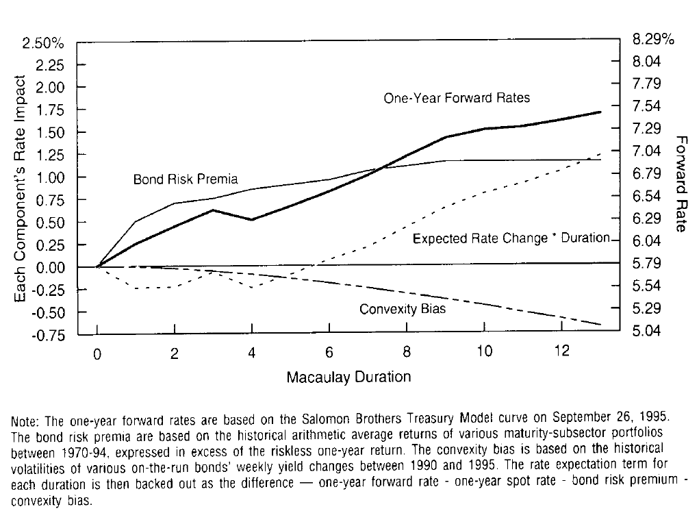
Figure 2 Decomposing Forward Rates Into Their Components, Using Historical Average Risk Premia and Volatilities

If bond risk premia vary over time, the use of historical average risk premia may be misleading. As an alternative, we can use survey data or rate predictions based on a quantitative forecasting model to proxy for the market's rate expectations. In Figure 3, we use the consensus interest rate forecasts from the Blue Chip Financial Forecast to proxy for the market's rate expectations. In addition, we use implied volatilities from option prices to compute the convexity bias. These components can be used together with the one-year forward rates to back out estimates of the unobservable bond risk premia.

如果债券风险溢价随时间而变化，使用历史平均风险溢价可能会产生误导。作为替代，我们可以使用调查数据或基于量化预测模型的收益率预测来代替市场的收益率预期。在图3中，我们使用“Blue Chip金融预测”的一致收益率预测来代替市场的收益率预期。此外，我们使用期权价格的隐含波动率来计算凸度偏差。这些组成部分可以与一年期远期收益率一起使用，推算不可观察的债券风险溢价的估计。

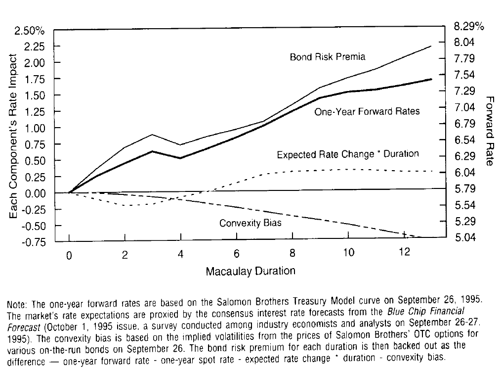
Figure 3 Decomposing Forward Hates Into Their Components, Using Survey Hate Expectations and Implied Volatilities

A comparison of Figures 2 and 3 shows that the two decompositions look similar up to the seven-year duration, but quite different beyond that point. The similarity of the convexity bias components in these two figures suggests that the use of historical or implied volatilities makes little difference, at least in this case. It is also clear that the Blue Chip survey predicted small declines in the short rates and small increases in the long rates, just as the inferred rate expectations in Figure 2. However, the predicted increases in long rates were smaller in this survey (where the largest increase was four basis points) than the inferred forecasts of Figure 2 (where the largest increase was eight basis points). Because the forward rate curve is the same in both figures, the smaller predicted rate increases lead to higher bond risk premia in Figure 3 than in Figure 2.^[4]

图2和图3的比较显示，两个分解从七年久期开始看起来类似，但是七年久期之前差别比较大。这两幅图中的凸度偏差部分的相似性表明，使用历史或隐含波动率几乎没有什么区别，至少在这个例子的情况下。很明显，Blue Chip调查预测短期收益率小幅下滑，长期收益率小幅上涨，正如图2推测的收益率预期一样。然而，本次调查中长期收益率的预测上升幅度（最大增幅为4个基点）小于图2的预测上升幅度（最大增幅为8个基点）。由于两个图中的远期收益率曲线相同，所以较小的预测收益率上升导致图3中的债券风险溢价高于图2。

Figures 2 and 3 are snapshots of the forward rates and their components on one date. A comparison of similar decompositions over time would provide insights into the relative variability of each component. In Figure 4, we try to illustrate the impact of changing rate expectations and risk premia on the steepness of the US Treasury bill curve. The figure shows that on four recent dates the forwards always implied larger increases in the three-month rate than the market expected, based on surveys of bond market analysts. The difference is proportional to the required bond risk premium of longer bills over shorter bills (because bills exhibit negligible convexity, its impact can be ignored). Not surprisingly, this difference is always positive; moreover, it varies over time.

图2和图3是某一天的远期收益率及其组成部分的截图。随着时间的推移，类似分解的比较将提供每个组成部分的相对变化的见解。在图4中，我们试图说明预期收益率变化和风险溢价对美国国库券曲线陡峭程度的影响。该数字显示，根据债券市场分析师的调查，近期四个交易日始终表明，三月期收益率相比于市场预期大幅上涨。差额与长期国库券超出短期国库券的债券风险溢价成比例（因为国库券的凸度影响可以忽略）。毫不奇怪，这种差异总是正的；此外，它随时间而变化。

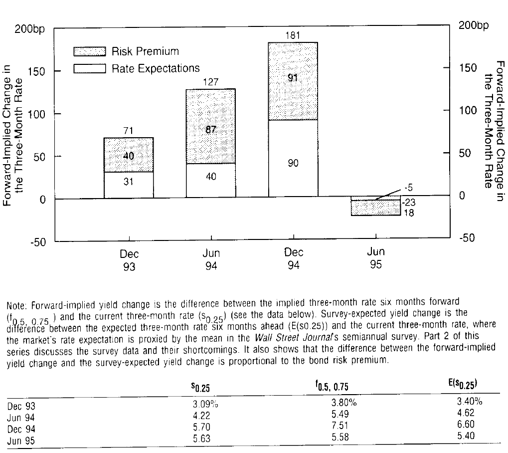
Figure 4 Forward Implied Yield Changes versus Survey-Expected Yield Changes in the Treasury Bill Market, 1993-95

The time-variation in the bond risk premium in Figure 4 appears economically reasonable. In December 1993, after a long bull market, market participants were complacent, neither expecting much higher rates nor demanding much compensation for duration extension. After the Fed began to tighten the monetary policy, the market expected further rate increases. In addition, the increase in volatility and in risk aversion levels (perhaps caused by own losses as well as the well-publicized losses of other investors) increased the required bond risk premia. By the end of 1994, the market was extremely bearish, expecting almost 100 basis points higher three-month rates in six months. However, the forwards were implying almost 200 basis points higher rates —— the difference reflects an abnormally large risk premium. In 1995, the bond market rallied strongly as the market's expectations for further Fed tightening receded and turned into expectations of easing policy. However, a large part of this rally was caused by the collapse in the required bond risk premium, perhaps reflecting lower inflation uncertainty and higher wealth that reduced the market's risk perceptions and risk aversion. In general, the time-variation in required returns appears to have contributed as much to the changing slope of the yield curve as has the time-variation in the market's interest rate expectations.^[5] Finally, we note that the time-variation in the estimated bond risk premia has been very market-directional over the past two years; this may not always be the case.

图4中债券风险溢价的时变性似乎在经济上是合理的。1993年12月，经过长时间的牛市，市场参与者非常满足，既不期望更高的收益率，也不要求增加久期。美联储开始收紧货币政策后，市场预期收益率进一步上调。此外，波动率和风险规避水平的增加（可能由自身的损失以及其他投资者的广泛的损失引起）提高了债券风险溢价。到1994年底，市场十分悲观，在六个月内预期三月期收益率涨幅将近100个基点。然而，远期收益率隐含涨幅高于近200个基点，差异反映出风险溢价异常大。1995年，债券市场强劲反弹，市场对美联储进一步紧缩政策的预期下降，并转为预期放松政策。然而，这个反弹的很大一部分是由于债券风险溢价的崩溃所致，也许是反映了更低的通胀不确定性和更高的财富，从而降低了市场的风险认知和风险规避。一般来说，所需回报的时变性似乎对收益率曲线的斜率变化有很大的作用，这与市场收益率预期的时变性一样。最后，我们注意到，债券风险预期的时变性在过去两年中表现出很强的市场方向性；这可能并非总是如此。

DECOMPOSING EXPECTED RETURNS OF BOND POSITIONS

分解债券头寸的预期回报

Five Alternative Expected Return Measures

五种预期回报度量方法

Our framework for decomposing the yield curve also provides a framework for systematic relative value analysis of government bonds with known cash flows. We can evaluate all bond positions' expected returns comprehensively, yet with simple and intuitive building blocks. We emphasize that relative value analysis should be based on near-term expected return differentials, not on yield spreads, which are only one part of them. That is, total return investors should care more about expected returns than about yields. Thus, our approach brings fixed-income investors closer to mean-variance analysis in which various positions are evaluated based on the trade-off between their expected return and return volatility.

我们分解收益率曲线的框架也为已知现金流的政府债券的相对价值分析提供了系统性框架。我们可以用简单直观的模块全面评估所有债券头寸的预期回报。我们强调，相对价值分析应以近期预期回报差异为基础，而不是利差，利差仅作为近期预期回报差的一部分。也就是说，总回报投资者应该更多关注预期回报而不是收益率。因此，我们的方法使固定收益投资者更熟悉均值-方差分析，根据预期回报和回报波动率之间的权衡来评估各种头寸。

Equation (1) shows that a zero's holding-period return is a sum of its return given an unchanged yield curve and its return caused by the changes in the yield curve. The return given an unchanged yield curve is called the rolling yield because it is a sum of the zero's yield and the rolldown return. The return caused by changes in the yield curve can be approximated well by duration and convexity effects. Taking expectations of Equation (1) and splitting the rolling yield into yield income and rolldown return, the near-term expected return of a zero is:

等式（1）表明零息债券持有期回报是给定不变收益率曲线情况下的回报及收益率曲线变化引起的回报之和。给定不变收益率曲线情况下的回报被称为滚动收益率，因为它是零息债券收益率和下滑回报之和。由收益率曲线变化引起的回报可以通过久期和凸度很好地近似。对等式（1）求期望，将滚动收益率分解为收益率回报和下滑回报，零息债券近期预期回报为：

\[\begin{aligned} \text{Expected return} &\approx \text{Yield income} \\ &+ \text{Rolldown return} \\ &+ \text{Value of convexity} \\ &+ \text{Expected capital gain/loss from the rate "view"} \end{aligned} \tag{3} \]

For details, see Equation (9) in Appendix A or the notes below Figure 5. A similar relation holds approximately for coupon bonds, and we will describe the three-month expected return of some on-the-run Treasury bonds as the sum of the four components in the right-hand side of Equation (3).^[6]

详情请参见附录A中的等式（9）或图5下面的附注。类似的关系对付息债券近似成立，我们将把一些活跃国债的三个月预期回报分解成等式（3）右侧的四个分量。

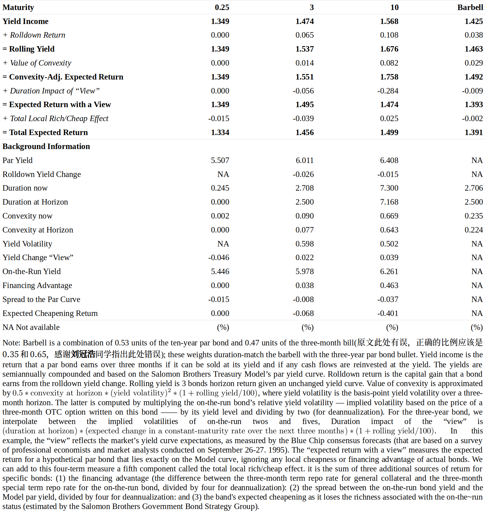
Figure 5 Three-Month Expected Return Measures and Their Components, as of 26 Sep 95

This framework is especially useful when evaluating positions of two or more government bonds, such as duration-neutral barbells versus bullets. We first compute expected return separately for each component and then compute the portfolio's expected return by taking a market-value weighted average of all the components' expected returns.

当评估两个或多个政府债券的头寸时，这种框架特别有用，例如久期中性的杠铃组合与子弹组合。我们首先针对每个分量分别计算预期回报，然后通过对所有分量的预期回报进行市值加权平均来计算投资组合的预期回报。

It may be helpful to show step by step how the expected return measures are improved, starting from simple yields and moving toward more comprehensive measures.

通过逐步展示如何从简单的收益率到更全面的方法来改进预期回报的度量，可能会对读者有所帮助。

• A bond's yield income includes coupon income, accrued interest and the accretion/amortization of price toward par value. Yield to maturity is the correct return measure if all interim cash flows can be reinvested at the yield and the bond can be sold at its purchasing yield.^[7] Yield ignores the rolldown return the bond earns if the yield curve stays unchanged.

• 债券的收益率回报包括息票收入、应计利息和价格对面值的增加/摊销。如果所有中期现金流可以以到期收益率再投资，债券可以以其购买时的收益率出售，则到期收益率是正确的回报率。如果到期收益率曲线保持不变，收益率将忽略下滑回报。

• Rolling yield is a better expected return proxy if an unchanged curve is a reasonable base case. Yet, it ignores the value of convexity and, thus, implicitly assumes no rate uncertainty. Thus, the rolling yield measures expected return if no curve change and no volatility is expected.

• 如果曲线不变，滚动收益率能更好地代表预期回报。然而，它忽略了凸度价值，因此隐含地假定收益率不存在不确定性。因此，如果没有曲线变化并且没有预期波动，则滚动收益率可以度量预期回报。

• Combining the rolling yield with the value of convexity improves the expected return measure further. In Part 5 of this series, we showed that a bond's convexity-adjusted expected return equals the sum of the rolling yield and the value of convexity. This measure recognizes the impact of rate uncertainty but implies that no change is expected in the yield curve. Empirical evidence described in Part 2 suggests that an unchanged yield curve is often a reasonable base "view".

• 将滚动收益率与凸度价值结合，进一步优化对预期回报的度量。在本系列的第5部分中，我们表明，债券的凸度调整预期回报等于滚动收益率与凸度价值的总和。这一度量方法认识到收益率不确定性的影响，但同时预期收益率曲线不会发生变化。第2部分的实证证据表明，收益率曲线不变通常是一个合理的基本“观点”。

• If investors want, they can replace the prediction of an unchanged curve with some other rate (or spread) "view". One possibility is to use survey-based information of the market's current rate forecasts; such an approach may be useful for backing out the market's required return for each bond. Alternatively, investors may ignore the market view and input either their own rate views or an economist's subjective rate forecasts or rate predictions from some quantitative model. For example, the predictors identified in Part 4 of this series can be used to forecast the changes in the long rates. The impact of any rate view is approximated by the expected yield change sealed by duration (see Equation (10) in Appendix A), which may be added to the convexity-adjusted expected return. The sum gives us the "expected return with a view" —— the four-term expected return measure in Equation (3). However, this equation is a perfect description of expected returns only for bonds that lie on the fitted curve. Thus, the relative value measures above ignore "local" or bond-specific richness or cheapness relative to the curve.

• 如果投资者想要，他们可以用一些其他收益率（或利差）观点替代不变曲线的预测。一种可能的方法是使用基于调查的市场收益率预测的信息，这种方法可能有助于推算出市场对每个债券所要求的回报。或者，投资者可以忽视市场观点，并从一些经济学家的主观预测或量化模型的预测中得到观点。例如，本系列第4部分中确定的预测因子可用于预测长期收益率的变化。任何收益率观点的影响都是由久期结合预期收益率变化近似（见附录A中的等式（10）），可以将其加到凸度调整后的预期回报中。这个总和给了我们“带观点的预期回报”——等式（3）中的四项预期回报度量。然而，这个等式是对落在拟合曲线上的债券预期回报的完美描述。因此，上述相对价值度量忽略了债券相对于曲线“局部的”或债券特定的估值偏差。

• Many technical factors can make a specific bond "locally" rich or cheap (relative to adjacent-maturity bonds), or they can make a whole maturity sector rich or cheap relative to the fitted curve. Such factors include supply effects (temporary price pressure on a sector caused by new issuance), demand effects (maturity limitations or preferences of important market participants —— for example, the richness of quarter-end bills), liquidity effects (lower transaction costs for on-the-runs versus off-the-run, for 30-year bonds versus 25-year bonds, for Treasury bills versus duration-matched coupon bonds, etc.), coupon effects (motivated by tax benefits, accounting rules, etc.), and above all, the financing effects (the "special" repo income that is common for on-the-runs).^[8] Fortunately, it is easy to add to the four-term expected return measures the financing advantage and two local cheapness measures —— the spread off the fitted curve and the expected cheapening toward the fitted curve. The five-term expected return measures are comprehensive measures of total expected returns —— ignoring small approximation errors, they incorporate all sources of expected return for noncallable government bonds.^[9]

• 许多技术因素可以使特定债券局部地高估或低估（相对于相邻到期债券），或者使整个期限区间相对于拟合曲线高估或低估。这些因素包括供给效应（由新发行造成的暂时的价格压力）、需求效应（期限限制或重要市场参与者的偏好，例如季末国库券的被高估）、流动性效应（例如活跃券对不活跃券、30年期债券对25年期债券、国库券对久期匹配的付息债券而言具有较低的交易成本）、票息效应（由税收优惠、会计规则等引发）、最重要的是融资效应（对活跃券而言常见的“特殊”回购回报）。幸运的是，很容易将融资优势和两个局部的低估度量（与拟合曲线的利差，相对于拟合曲线的预期低估量）添加到四因子预期回报度量中。五因子预期回报度量是预期回报总量的综合度量指标（忽略了小的近似误差），它们包含了非可赎回的政府债券所有预期回报来源。

As a numerical illustration, Figure 5 shows the various expected return measures for three bonds (the three-month Treasury bill and the three-year and ten-year on-the-run Treasury notes) and for the barbell combination of the three-month bill and the ten-year bond. In this example, we use as much market-based data as possible: for example, implied volatilities, not historical, to estimate the value of convexity, and the "view" (rate predictions) based on survey evidence of the market's rate expectations, not on a quantitative forecasting model. All the numbers are based on the market prices as of September 26, 1995.

作为数值例子，图5显示了三种债券（三月期国库券、三年期和十年期国债）以及三月期国库券-十年期债券杠铃组合的各种预期回报度量。在这个例子中，我们使用尽可能多的基于市场的数据：例如，用隐含波动率而不是历史波动率来估计凸度价值，以及基于市场收益率预期的调查证据而不是量化预测模型形成的收益率“观点”（收益率预测）。所有数字都是根据1995年9月26日的市场价格计算的。

The top panel of Figure 5 shows how nicely the different components of expected returns can be added to each other. Moreover, the barbell's expected return measures are simply the market-value weighted averages of its components' expected returns. In this case, the yield income, the rolldown return and the value of convexity are all higher for the longer bonds. In contrast, the duration impact of the market's rate view is negative, because the Blue Chip survey suggested that the market expected small increases in the three-year and the ten-year rates over the next quarter. The local rich/cheap effect is negative for the shorter instruments but positive for the ten-year note; the reason is that the negative yield spread and the expected cheapening of the ten-year note are not sufficient to offset the ten-year note's high repo market advantage. According to all five expected return measures, the barbell has a lower expected return than the duration-matched bullet.

图5的上半部分显示了预期回报的不同组成部分可以如何更好地相互添加。此外，杠铃组合的预期回报度量只是其组成部分预期回报的市值加权平均。在这种情况下，长期债券的收益率回报、下滑回报和凸度价值均较高。相比之下，市场收益率观点的久期影响是负的，因为Blue Chip调查显示，市场预期下个季度的三年期和十年期收益率将小幅上涨。局部高估/低估效应对于期限较短的国库券为负数，但对十年期债券为正，原因是负的利差和预期十年期债券被低估的程度不足以抵消十年期债券在回购市场的优势。根据所有五项预期回报度量，杠铃组合的预期回报比久期匹配子弹组合低。

Figure 6 shows the five different expected return curves plotted on the three bonds' durations. In this case, the simplest expected return measure (yield income) and the most comprehensive measure (total expected return) happen to be quite similar. In general, the relative importance of the five components may be dramatically different from that in Figure 5 where the yield income dominates. The longer the asset's duration and the shorter the investment horizon, the greater is the relative importance of the duration impact. It is worth noting that realized returns can be decomposed in the same way as the expected returns and that the duration impact typically dominates the realized returns even more.^[10]

图6显示了在三个债券关于久期绘制的五种不同的预期回报曲线。在这种情况下，最简单的预期回报度量（收益率回报）和最全面的度量（总预期回报）恰恰相当。一般来说，五个组成部分的相对重要性可能与图5中收益率回报占主导地位的情况有显着差异。资产久期越长、投资期限越短，久期影响的相对重要性就越大。值得注意的是，实现的回报可以以与预期回报相同的方式分解，久期的影响通常更多主导实现的回报。

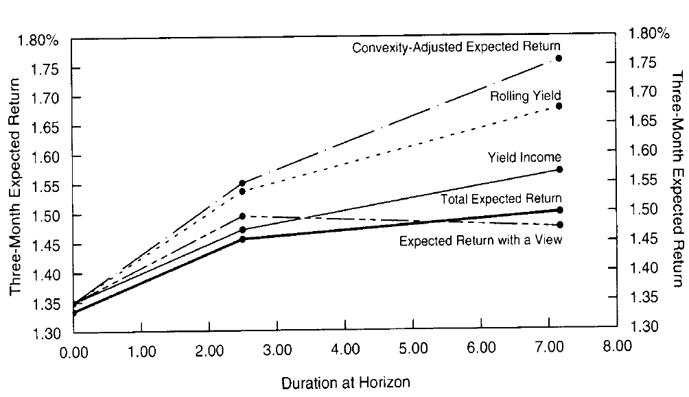
Figure 6 Expected Returns at a Three-Month Bill, a Three-Year Bond and a Ten-Year Bond, as of 26 Sep 95

The total expected returns, if estimated carefully, should produce the most useful signals for relative value analysis because they include all sources of expected returns. Yield spreads may be useful signals, but they are only a part of the picture. Therefore, we advocate the monitoring of broader expected return measures relative to their history as cheapness indicators —— just as yield spreads are often monitored relative to their history.

如果仔细估计，总预期回报应该产生最有用的相对价值分析信号，因为它们包括所有预期回报来源。利差可能是有用的信号，但它们只是一部分。因此，我们主张监测预期回报度量相对于其历史水平的差异作为低估指标，正如通常监测利差相对于其历史水平的差异一样。

The components of expected returns discussed above are not new. However, few investors have combined these components into an integrated framework and based their historical analysis on broad expected return measures. An additional useful feature of this framework is that all types of government bond trades can be evaluated consistently within it: the portfolio duration decision (market-directional view); the maturity-sector positioning and barbell-bullet decision (curve-reshaping view); and the individual issue selection (local cheapness view). With small modifications, the framework can be extended to include the cross-country analysis of currency-hedged government bond positions. Other possible future extensions include the analysis of foreign exchange exposure and the analysis of spread positions between government bonds and other fixed-income assets.

上述关于预期回报的组成部分的讨论并不新鲜。然而，很少有投资者将这些组成部分组合成一个综合框架，并将他们的历史分析基于广泛的预期回报度量之上。这个框架的一个额外的功能是所有类型的政府债券交易可以在其中一致地评估：投资组合久期的制定（市场的方向性观点）；期限配比和杠铃-子弹组合的制定（曲线形变观点）和个券选择的制定（局部低估观点）。经过少量修改，可以将框架扩大到包括货币对冲的跨国政府债券头寸的分析。其他可能的未来扩展包括外汇敞口分析以及政府债券与其他固定收益资产之间的利差分析。

We note some reservations. Even if two investors use the same general framework and the same type of expected return measure, they may come up with different numbers because of different data sources and different estimation techniques.

我们注意到一些遗留问题。即使两个投资者使用相同的一般框架和相同的预期回报度量，也可能会因为不同的数据来源和不同的估算技术而产生不同的结果。

• The whole analysis can be made with any raw material; we emphasize the importance of good-quality inputs. Various candidates for the raw material include on-the-run and off-the-run government bonds, STRIPS, Eurodeposits, swaps, and Eurodeposit futures. This multitude of course opens the possibility of trading between these curves if we can assess how various characteristics (say, convexity) are priced in each curve. The most common approach is first to estimate the spot curve (or discount function) using a broad universe of coupon government bonds as the raw material, and then to compute the forward rates and other relevant numbers. In European bond markets, the liquid swap curve (using cash Eurodeposits and swaps as the raw material) has gained more of a benchmark status. Of course, some credit and tax-related spread may exist between the swap curve and the government bond yield curve. Recently, yet another approach has become popular: Eurodeposit futures prices are used as the raw material. In this case, the forward rates are computed by adjusting for the convexity difference between a futures contract and a forward contract, and only then are spot rates computed from the forwards.

• 整个分析可以用任何原始资料进行，我们强调输入优质数据的重要性。原始资料包括活跃和不活跃的政府债券、零息债券（STRIPS）、欧洲存款、互换和欧洲存款期货。当然，如果我们能够评估每个曲线中的各种特性（如凸度）是如何定价的，那么很大程度上可以提供这些曲线之间交易的可能性。最常见的做法是首先用广泛的付息政府债券作为原始资料估算即期收益率曲线（或贴现函数），然后计算远期收益率和其他相关数字。在欧洲债券市场，流动性好的互换曲线（以现金欧洲存款和互换为原始资料）已经更多地最为基准。当然，互换曲线和政府债券收益率曲线之间可能存在一些信用和税收相关的利差。最近，另一种方法已经变得流行起来：以欧元存货期货价格为原始资料。在这种情况下，远期收益率是通过调整期货合约与远期合约之间的凸度差来计算的，然后才是从远期收益率计算的即期收益率。

• Some components of expected returns are easier to measure —— and less debatable —— than others. The yield income is relatively unambiguous. The rolldown return and the local rich/cheap effects depend on the curve-fitting technique. The value of convexity depends on the volatility input and, thus, on the volatility estimation technique. The rate "view," the fourth term, can be based on various approaches, such as quantitative modeling or subjective forecasting that relies on fundamental or technical analysis. Even the quantitative approach is not purely objective because infinitely many alternative forecasting models and estimation techniques exist. Forecasting rate changes is of course the most difficult task as well as the one with greatest potential rewards and risks. Forecasting changes in yield spreads may be almost as difficult. The short-term returns of most bond positions depend primarily on the duration impact (rate changes or spread changes). However, even if investors cannot predict rate changes, they may earn superior returns in the long run —— and with less volatility —— by systematically exploiting the more stable sources of expected return differentials across bonds: yields; rolldown returns; value of convexity; and local rich/cheap effects. More generally, while the total expected return differentials are, in theory, better relative value indicators than the yield spreads, in practice, measurement errors conceivably can make them so noisy that they give worse signals. Therefore, it is important to check with historical data that any supposedly superior relative value tools would have enhanced the investment performance at least in the past.

• 预期回报的一些组成部分比其他部分更容易度量。收益率回报相对明显。下滑回报和局部高估/低估效应取决于曲线拟合技术。凸度价值取决于波动率，因此取决于波动率估计技术。第四项——收益率“观点”，可以基于各种方法得到，例如依赖于基本面或技术分析的量化模型和主观预测。即使是量化方法也不是纯粹客观的，因为存在无数多个替代预测模型和估计技术。预测收益率变化当然是最困难的任务，也是最有潜在回报和风险的。预测利差变化可能几乎同样困难。大多数债券头寸的短期回报主要取决于久期的影响（收益率或利差变化）。然而，即使投资者无法预测收益率变动，长期而言也可能获得较高的回报和较小的波动率——通过系统地挖掘更稳定的，不同债券的预期回报差异的来源：收益率回报、下滑回报、凸度价值和局部高估/低估的影响。更一般地说，虽然总预期回报差异在理论上是比利差更好的相对价值指标，但在实践中，测量误差可以使它们的噪声很大，进而产生更差的交易信号。因此，重要的是要用历史数据来检验，任何所谓优越的相对价值工具，至少在过去都能提高投资业绩。

Link to Scenario Analysis

与情景分析相联系

Many active investors base their investment decisions on subjective yield curve views, often with the help of scenario analysis. Our framework for relative value analysis is closely related to scenario analysis. It may be worthwhile to explore the linkages further.

许多积极的投资者借助情景分析的帮助，将他们的投资决策建立在收益率曲线的主观观点上。我们的相对价值分析框架与情景分析密切相关。可能值得进一步探讨联系。

An investor can perform the scenario analysis of government bonds in two steps. First, the investor specifies a few yield curve scenarios for a given horizon and computes the total return of his bond portfolio —— or perhaps just a particular trade —— under each scenario. Second, the investor assigns subjective probabilities to the different scenarios and computes the probability-weighted expected return for his portfolio. Sometimes the second step is not completed and investors only examine qualitatively the portfolio performance under each scenario. However, we advocate performing this step because investors can gain valuable insights from it. Specifically, the probability-weighted expected return is the "bottom-line" number a total return manager should care about. By assigning probabilities to scenarios, investors also can explicitly back out their implied views about the yield curve reshaping and about yield volatilities and correlations.

投资者可以分两步进行政府债券的情景分析。首先，投资者在给定的期限内指定了一些收益率曲线情景，并计算每个情景下债券投资组合的总回报，或者也可能只是特定的交易。第二，投资者将主观概率分配给不同的情景，并计算其投资组合的概率加权预期回报。有时候第二步不需要完成，投资者只会在每个情景下定性地检查投资组合的表现。但是，我们主张执行这一步，因为投资者可以从中获得宝贵的见解。具体来说，概率加权的预期回报是总回报经理应该关心的“底线”数字。通过将概率分配给情景，投资者也可以明确地推算出其关于收益率曲线形变以及关于收益率波动率和相关系数的隐含观点。

In scenario analysis, investors define the mean yield curve view and the volatility view implicitly by choosing a set of scenarios and by assigning them probabilities. In contrast, our framework for relative value analysis involves explicitly specifying one yield curve view (which corresponds to the probability-weighted mean yield curve scenario) and a volatility view (which corresponds to the dispersion of the yield curve scenarios). Either way, the yield curve view determines the duration impact and the volatility view determines the value of convexity (and these views together approximately define the expected yield distribution).

在情景分析中，投资者通过选择一组情景并分配其概率来隐含地定义平均曲线观点和波动率观点。相比之下，我们的相对价值分析框架包括明确指定一个收益率曲线观点（对应于概率加权的平均曲线情景）和波动率观点（其对应于收益率曲线情景的分散程度）。无论哪种方式，收益率曲线观点决定久期影响，波动率观点确定凸度价值（这些观点一起大概界定了预期收益率分布）。

Figure 7 presents a portfolio that consists of five equally weighted zero-coupon bonds with maturities of one to five years and (annually compounded) yields between 6% and 7%. The portfolio's maturity, and its Macaulay duration —— initially is three years. Over a one-year horizon, each zero's maturity shortens by one year. We specify five alternative yield curve scenarios over the horizon: parallel shifts of +100 basis points and -100 basis points; no change; a yield increase combined with a curve flattening; and a yield decline combined with a curve steepening (see Figure 8). We compute the one-year holding-period returns for each asset and for the portfolio under each scenario. In particular, the neutral scenario shows the rolling yield that each zero earns if the yield curve remains unchanged. We can evaluate each scenario separately. However, such analysis gives us limited insight —— for example, the last column in Figure 7 shows just that bearish scenarios produce lower portfolio returns than bullish scenarios.

图7显示了一个投资组合，其中包括五个等权的零息债券，期限为一至五年，收益率（每年复利）在6%至7%之间。投资组合的期限及其Macaulay久期最初为三年。在一年的期限内，每个零息债券的期限将缩短一年。我们在持有期内指定了五种可能的收益率曲线情景：平移+100个基点和-100个基点、不变、收益率增加与曲线变平相结合、收益率下降与曲线变陡相结合（见图8）。我们计算每种情景下每种资产和投资组合的一年持有期回报。特别地，如果收益率曲线保持不变，则中性情景显示每个零息债券的滚动收益率。我们可以分别评估每个情景。然而，这样的分析给我们提供了有限的洞察力——仅仅是熊市情景产生的投资组合回报比牛市情景更低，正如图7中的最后一列栏显示的。

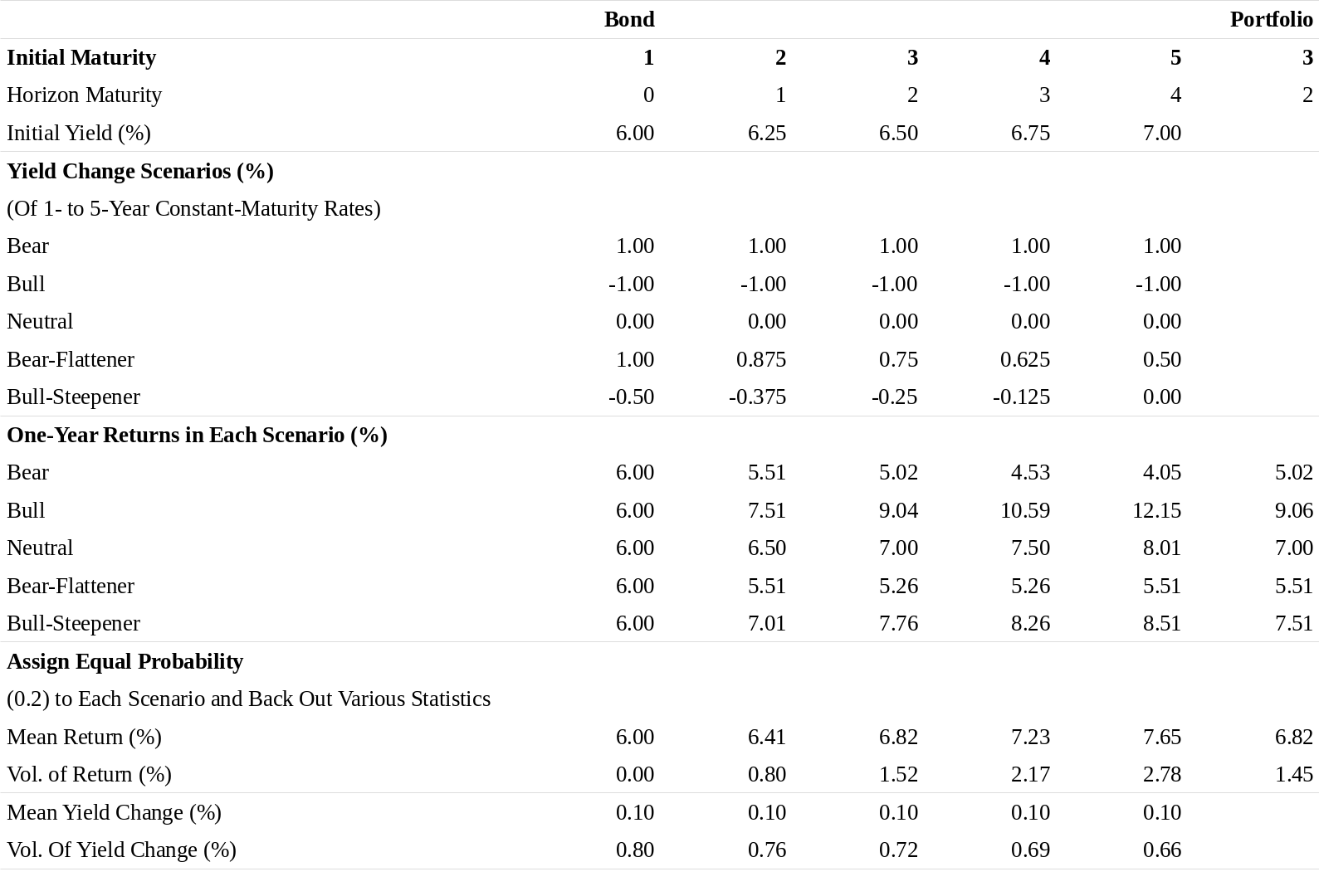
Figure 7 Scenario Analysis and Expected Band Returns

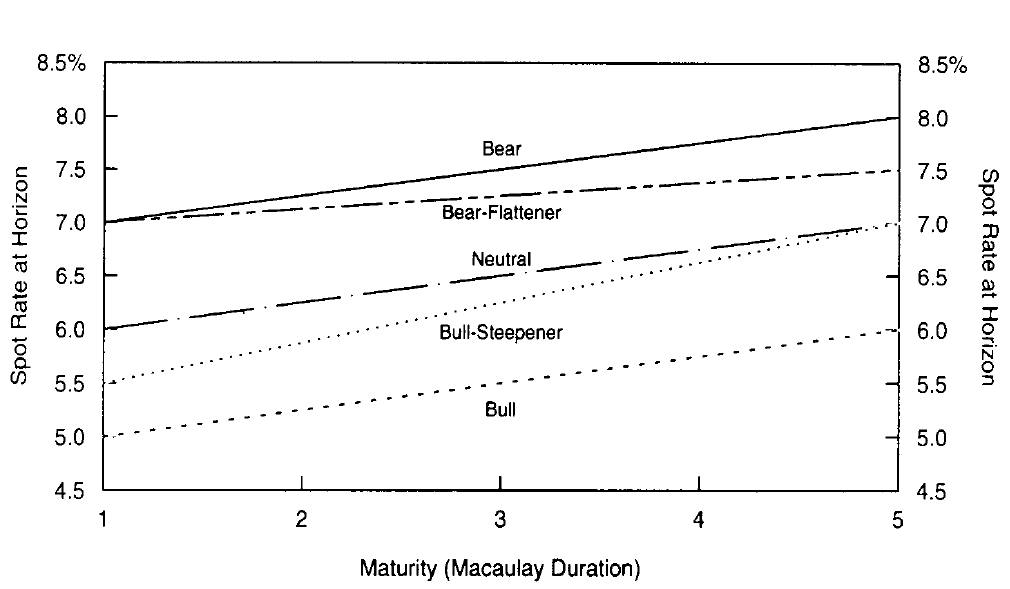
Figure 8 Various Yield Curve Scenarios

In contrast, if we assign probabilities to the scenarios, we can back out many numbers of potential interest. We begin with a simple example in which we only use the two first scenarios, parallel shifts of 100 basis points up or down. If we assign these scenarios equal probabilities (0.5), the expected return of the portfolio is 7.04% (\(=0.5*5.02 + 0.5*9.06\)). On average, these scenarios have no view about curve changes; yet, this expected return is four basis points higher than the expected portfolio return given no change in the curve (that is, the 7% rolling yield computed in the neutral scenario). This difference reflects the value of convexity. If we only use one scenario, we implicitly assume zero volatility, which leads to downward-biased expected return estimates for positively convex bond positions. If we use the two first scenarios (bear and bull), we implicitly assume a 100-basis-point yield volatility; this assumption may or may not be reasonable, but it certainly is more reasonable than an assumption of no volatility. This example highlights the importance of using multiple scenarios to recognize the value of convexity. (The value is small here, however, because we focus on short-duration assets that have little convexity.)

相比之下，如果我们将概率分配给情景，我们可以推算出许多潜在的有趣观点。我们从一个简单的例子开始，只使用前两个情景：上下平移100个基点。如果我们分配这些情景相等概率（0.5），投资组合的预期回报为7.04%（\(=0.5*5.02 + 0.5*9.06\)）。平均而言，这些情景认为曲线没有变化。然而这一预期回报高于曲线没有变化情境下的预期回报四个基点（即在中性情景中计算出的7%滚动收益率）。这个差异反映了凸度价值。如果我们只使用一种情景，我们隐含地假定零波动率，这导致了正凸度债券头寸的预期回报的被低估。如果我们使用前两个情景（熊市和牛市），我们隐含地假设100个基点的收益率波动率，这个假设可能合理也可能不合理，但是肯定比没有波动的假设更合理。此例强调了使用多个情景来识别凸度价值的重要性。（这里的凸度价值很小，是因为我们专注于几乎没有凸度的短久期资产。）

Now we return to the example with all five yield curve scenarios in Figure 8. As an illustration, we assign each scenario the same probability (\(p_i = 0.2\)). Then, it is easy to compute the portfolio's probability-weighted expected return:

现在我们回到图8中所有五个收益率曲线情景的例子。作为一个例证，我们为每个情景分配相同的概率（\(p_i = 0.2\)）。那么，很容易计算投资组合的概率加权预期回报：

\[E(h_p) = \sum_{i=1}^5 p_i * h_i = 0.2*(5.02+9.06+7.00+5.51+7.51) = 6.82 \tag{4} \]

Given these probabilities, we can compute the expected return for each asset, and it is possible to back out the implied yield curve views. The lower panel in Figure 7 shows that the mean yield change across scenarios is +10 basis points for each rate (because the bear-flattener and the bull-steepener scenarios are not quite symmetric in magnitude in this example), implying a mild bearish bias but no implied curve-steepness views. In addition, we can back out the implied basis-point yield volatilities (or return volatilities) by measuring how much the yield change (or return) outcomes in each scenario deviate from the mean. These yield volatility levels are important determinants of the value of convexity. The last line in Figure 7 shows that the volatilities range from 80 to 66 basis points, implying an inverted term structure of volatility. Finally, we can compute implied correlations between various-maturity yield changes; the curve behavior across the five scenarios is so similar that all correlations are 0.92 or higher (not shown). Note that all correlations would equal 1.00 if only the first three scenarios were used; the imperfect correlations arise from the bear-flattener and the bull-steepener scenarios.

考虑到这些概率，我们可以计算每个资产的预期回报，并且可以推算出隐含的收益率曲线观点。图7中的下半部分显示，不同情景的平均收益率变化为+10个基点（因为在这个例子中，熊平和牛陡的情景在大小上不是很对称），这意味着温和的看跌偏差但没有隐含曲线变陡的观点。此外，我们可以通过测量每种情况下的收益率变化（或回报）结果与平均值的偏差多少来推算隐含的基点收益率波动率（或回报波动率）。这些收益率波动率水平是凸度价值的重要决定因素。图7的最后一行显示，波动率幅度在80到66个基点之间，这意味着波动率期限结构的倒挂。最后，我们可以计算不同期限收益率变化之间的隐含相关性，五个情景中的曲线行为非常相似，所有相关性均为0.92或更高（未显示）。注意，如果仅使用前三种情况，所有相关性将等于1.00；这种不完全的相关性来自于熊平和牛陡情景。

Whenever an investor uses scenario analysis, he should back out these implicit curve views, volatilities and correlations —— and check that any biases are reasonable and consistent with his own views. Without assigning the probabilities to each scenario, this step cannot be completed; then, the investor may overlook hidden biases in his analysis, such as a biased curve view or a very high or low implicit volatility assumption which makes positive convexity positions appear too good or too bad. If investors use quantitative tools —— such as scenario analysis, mean-variance optimization, or the approach outlined in this report —— to evaluate expected returns, they should recognize the importance of their rate views in this process. Strong subjective views can make any particular position appear attractive. Therefore, investors should have the discipline and the ability to be fully aware of the views that are input into the quantitative tool.

每当投资者使用情景分析时，他应该推算出这些隐含的曲线观点、波动率和相关性，并检查任何偏差是否合理和符合自己的观点。没有为每个情景分配概率，此步骤无法完成；那么投资者在分析中可能会忽视隐藏的偏差，比如有偏差的曲线观点，或是非常高或低的隐含波动率假设，这使得正凸度的头寸看起来太好或太差。如果投资者使用量化工具，例如情景分析，均值-方差优化或本报告中概述的方法来评估预期回报，那么他们应该在这个过程中认识到他们的收益率观点的重要性。强烈的主观观点可以使任何特定头寸显得有吸引力。因此，投资者应该具有纪律和能力充分认识纳入量化工具的（收益率）观点。

In addition to the implied curve views, we can back out the four components of expected returns discussed above. In this example, we only analyze bonds that lie “on the curve" and thus can ignore the fifth component, the local rich/cheap effects. (1) We measure the yield income from the portfolio by a market-value weighted average yield of the five zeros, which is 6.50% (see footnote 7). (2) Each asset's rolldown return is the difference between the horizon return given an unchanged yield curve and the yield income. Figure 7 shows that the horizon return for the portfolio is 7% in the neutral scenario; thus, the portfolio's (market-value weighted average) rolldown return is 50 basis points (= 7% - 6.5%). Note that the rolldown return is larger for longer bonds, reflecting the fact that the same rolldown yield change (25 basis points) produces larger capital gains for longer bonds. (3) The value of convexity for each zero can be approximated by \(0.5*\text{convexity at horizon}*(\text{basis-point yield volatility})^2*(1 + \text{rolling yield}/100)\). Using the implicit yield volatilities in Figure 7, this value varies between 0.6 and 4.5 basis points across bonds. The portfolio's value of convexity is a market-value weighted average of the bond-specific values of convexity, or roughly two basis points. (4) The duration impact of the rate "view" for each bond equals \((-\text{duration at horizon})*(\text{expected yield change})*(1 + \text{rolling yield}/100)\). The last term is needed because each invested dollar grows to \((1 + \text{rolling yield}/100)\) by the end of horizon when the repricing occurs. The core of the duration impact is the product of duration and expected yield change. The expected yield change refers to the change (over the investment horizon) in a constant-maturity rate of the bonds horizon maturity. In Figure 7, all rates are expected to increase by ten basis points, and the duration impact on specific bonds' returns varies between 0 and -40 basis points. The portfolio's duration impact is a market-value weighted average of bond-specific duration impacts, or about -20 basis points.^[11]

• 除了隐含的曲线观点外，我们还可以推算上面讨论的预期回报的四个组成部分。在这个例子中，我们只分析“曲线上的”债券，从而忽略了第五个组成部分，局部的高估/低估的影响。（1）我们通过五个零息债券的市值加权来衡量投资组合的收益率回报，即6.50%（见注7）；（2）每个资产的下滑回报是一个不变收益率曲线情况下的持有期回报与收益率回报之间的差，图7显示投资组合的持有期回报为7%。因此，投资组合（市值加权平均）下滑回报为50个基点（= 7% - 6.5%）。请注意，长期债券的下滑回报较大，反映出同样的收益率下滑变化（25个基点）对长期债券产生较大的资本回报；（3）每个零息债券的凸度价值可以近似为\(0.5*\text{期末凸度}*(\text{基点收益率波动率})^2*(1 + \text{滚动收益率}/100)\)；使用图7中的隐含收益率波动率，该值变化区间在0.6和4.5基点。投资组合的凸度价值是债券凸度价值的市值加权平均值，大致两个基点；（4）每个债券收益率“观点”的久期影响等于\((-\text{期末久期})*(\text{预期收益率变化})*(1 + \text{滚动收益率}/100)\)。最后一项是必要的，因为当重新定价发生时，每个投资美元在持有期末增长到\((1 + \text{滚动收益率}/100)\)。久期影响的核心是久期和预期收益率变化的乘积。预期收益率变动是指固定期限上的收益率变化（在投资期限内）。在图7中，所有收益率预期将增加10个基点，久期对特定债券回报的影响在0到-40个基点之间变化。投资组合的久期影响是特定债券久期影响的市值加权平均，约为-20个基点。

Figure 9 shows that the four components add up to the total probability-weighted expected return of 6.82%. Decomposing expected returns into these components should help investors to better understand their own investment positions. For example, they can see what part of the expected return reflects static market conditions and what part reflects their subjective market view. Unless they are extremely confident about their market view, they can emphasize the part of expected return advantage that reflects static market conditions. In our example, the duration effect is small because the implied rate view is quite mild (ten basis points) and the one-year horizon is relatively long (the "slower" effects have time to accrue). With a shorter horizon and stronger rate views, the duration impact would easily dominate the other effects.

图9显示，这四个组成部分加起来的总概率加权预期回报为6.82%。将预期回报分解为这些组成部分应有助于投资者更好地了解自己的头寸。例如，他们可以看到预期回报的哪一部分反映了静态市场状况，哪些部分反映了他们的主观市场观点。除非他们对市场观点非常有信心，否则他们可以强调反映静态市场条件的预期回报优势部分。在我们的示例中，久期效应很小，因为隐含的收益率观点相当温和（十个基点），一年的投资期限相对较长（“较慢”的影响有时间去逐渐累积）。如果投资期限更短，收益率观点更强，久期的影响将很容易超过其他的影响。

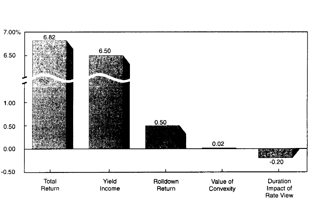
Figure 9 Decomposing the Total Expected Return into Four Components

APPENDIX A. DECOMPOSING THE FORWARD RATE STRUCTURE INTO ITS MAIN DETERMINANTS

附录A：将远期收益率结构分解为主要决定部分

In this appendix, we show how the forward rate structure is related to the market's rate expectations, bond risk premia and convexity bias. In particular, the holding-period return of an n-year zero-coupon bond can be described as a sum of its horizon return given an unchanged yield curve and the end-of-horizon price change that is caused by a change in the n-1 year constant-maturity spot rate (\(\Delta s_{n-1}\)). The horizon return equals a one-year forward rate, and the end-of-horizon price change can be approximated by duration and convexity effects. These relations are used to decompose near-term expected bond returns and the one-period forward rates into simple building blocks. All rates and returns used in the following equations are compounded annually and expressed in percentage terms.

在本附录中，我们展示了远期收益率结构与市场收益率预期、债券风险溢价和凸度偏差的关系。特别是，n年零息债券的持有期回报可以被描述为给定不变收益率曲线的持有期回报与n-1年期即期收益率引起的期末价格变动之和。持有期回报（不变曲线）等于一年期远期收益率，而期末价格变化可以由久期和凸度近似。这些关系用于将短期预期债券回报和一年期远期收益率分解为简单的模块。以下等式中使用的所有收益率和回报均为年化并以百分比表示。

\[\begin{aligned} \frac{h_n}{100} &= \frac{P^*_{n-1} - P_n}{P_n} = \frac{(P^*_{n-1} - P_{n-1}) + (P_{n-1} - P_n)}{P_n} \\ &= (\frac{\Delta P_{n-1}}{P_{n-1}} * \frac{P_{n-1}}{P_n}) + (\frac{P_{n-1}}{P_n} - 1), \end{aligned} \tag{5} \]

where \(h_n\) is the one-period holding-period return of an n-year bond, \(P_n\) is its price (today), \(P_{n-1}^*\) is its price in the next period (when its maturity is n-1), and \(\Delta P_{n-1} = P^*_{n-1} - P_{n-1}\). The second term on the right-hand side of Equation (5) is the bonds rolling yield (horizon return). The first term on the right-hand side of Equation (5) is the instantaneous percentage price change of an n-1 year zero, multiplied by an adjustment term \(P_{n-1}/P_n\).^[12]

其中\(h_n\)是n年期债券的一（年）期持有期回报，\(P_n\)为其当前价格（当下），\(P_{n-1}^*\)为其下一期（期限为n-1年）的价格，并且\(\Delta P_{n-1} = P^*_{n-1} - P_{n-1}\)。等式（5）右边第二项是滚动收益率（持有期回报）。等式（5）右边的第一项是n-1年零息债券的瞬时百分比价格变化乘以修正项\(P_{n-1}/P_n\)。

Equation (6) shows that the zero's rolling yield (\(P_{n-1} /P_n - 1\)) equals, by construction, the one-year forward rate between n-1 and n. Moreover, the adjustment term equals one plus the forward rate.

等式（6）表明零息债券的滚动收益率（\(P_{n-1} /P_n - 1\)）通过构造等于n-1年期和n期年之间的一年期远期收益率。此外，修正项等于一加上远期收益率。

\[1+ \frac{f_{n-1,n}}{100} = \frac{(1+\frac{s_n}{100})^n}{(1+\frac{s_{n-1}}{100})^{n-1}} = \frac{P_{n-1}}{P_n}. \tag{6} \]

Equation (7) shows the well-known result that the percentage price change (\(\Delta P / P\)) is closely approximated by the first two terms of a Taylor series expansion, duration and convexity effects.

公式（7）显示了价格变化百分比可以由泰勒级数展的前两项（久期和凸度）近似这一众所周知的结果。

\[100 * \frac{\Delta P}{P} \approx -Dur*(\Delta s) + 0.5 * Cx * (\Delta s)^2, \tag{7} \]

where \(Dur \equiv - \frac{dP}{ds}*\frac{100}{P}\) and \(Cx \equiv \frac{d^2P}{ds^2}*\frac{100}{P}\).

其中\(Dur \equiv - \frac{dP}{ds}*\frac{100}{P}\)，\(Cx \equiv \frac{d^2P}{ds^2}*\frac{100}{P}\)。

Plugging Equations (6) and (7) into (5), we get:

将等式（6）和等式（7）代入等式（5），得到：

\[h_n \approx f_{n-1,n} + (1+\frac{f_{n-1,n}}{100})*[-Dur_{n-1}*(\Delta s_{n-1}) + 0.5*Cx_{n-1}*(\Delta s_{n-1})^2]. \tag{8} \]

Even if the yield curve shifts occur during the horizon, for performance calculation purposes the repricing takes place at the end of horizon. This disparity causes various differences between the percentage price changes in Equations (7) and (8). First, the amount of capital that experiences the price change grows to (\(1+f_{n-1,n}/100\)) by the end of horizon. Second, the relevant yield change is the change in the n-1 year constant-maturity rate, not in the n-year zero's own yield (the difference is the rolldown yield change).^[13] Third, the end-of-horizon (as opposed to the current) duration and convexity determine the price change.

即使在持有期收益率曲线发生变化，为了表现计算需要，重新定价发生在持有期末。这种差异导致等式（7）和（8）中的价格变动百分比之间的各种差异。首先，经历价格变化的资本数量在持有期末逐渐增长到\(1+f_{n-1,n}/100\)。第二，相关收益率变化是n-1年期收益率的变化，而不是n年期收益率（差额是下滑收益率变动）。第三，期末（而不是当前）的久期和凸度决定了价格变动。

The realized return can be split into an expected part and an unexpected part. Taking expectations of both sides of Equation (8) gives us the n-year zero's expected return over the next year.

实现的回报可以分为预期部分和非预期部分。对等式（8）的两边求期望得到明年的n年期零息债券预期回报。

\[E(h_n) \approx f_{n-1,n} + (1+\frac{f_{n-1,n}}{100})*[-Dur_{n-1}*E(\Delta s_{n-1}) + 0.5*Cx_{n-1}*E(\Delta s_{n-1})^2]. \tag{9} \]

Recall from Equation (6) that the one-period forward rate equals a zero's rolling yield, which can be split to yield and rolldown return components. In addition, the expected yield change squared is approximately equal to the variance of the yield change or the squared volatility, \(E(\Delta s_{n-1})^2 \approx (Vol(\Delta s_{n-1}))^2\). This relation is exact if the expected yield change is zero. Thus, the zero's near-term expected return can be written (approximately) as a sum of the yield income, the rolldown return, the value of convexity, and the expected capital gains from the rate "view" (see Equation (3)).

回顾等式（6），一期远期收益率等于零息债券的滚动收益率，可以被分割为收益率回报和下降回报。此外，收益率变化平方的预期近似等于收益率变化方差或波动率平方（\(E(\Delta s_{n-1})^2 \approx (Vol(\Delta s_{n-1}))^2\)）。如果收益率变化的期望为零，则该关系是准确的。因此，零息债券的近期预期回报可以写成收益率回报、下滑回报、凸度价值和从“观点”得到的预期资本回报的总和（见公式（3））。

We can interpret the expectations in Equation (9) to refer to the market's rate expectations. Mechanically, the forward rate structure and the market's rate expectations on the right-hand side of Equation (9) determine the near-term expected returns on the left-hand side. These expected returns should equal the required returns that the market demands for various bonds if the market's expectations are internally consistent. These required returns, in turn, depend on factors such as each bond's riskiness and the market's risk aversion level. Thus, it is more appropriate to think that the market participants, in the aggregate, set the bond market prices to be such that given the forward rate structure and the consensus rate expectations, each bond is expected to earn its required return.^[14]

我们可以将等式（9）中的期望解释为市场的收益率预期。等式（9）右侧的远期收益率结构和市场收益率预期决定了左边的近期预期回报。如果市场预期内在一致，这些预期回报应等于市场对各种债券的所要求回报。这些所要求的回报反过来依赖于每个债券的风险水平和市场风险厌恶程度等因素。因此，更合适的观点是，市场参与者总体上依据远期收益率结构和一致收益率预期来设定债券市场价格，每个债券预期获得所要求的回报。

Subtracting the one-period riskless rate (\(s_1\)) from both sides of Equation (9), we get:

在等式（9）两端减去一年期无风险收益率（\(s_1\)）得到：

\[E(h_n - s_1) \approx f_{n-1,n} -s_1 + (1+\frac{f_{n-1,n}}{100})*[-Dur_{n-1}*E(\Delta s_{n-1}) + 0.5*Cx_{n-1}*(Vol(\Delta s_{n-1}))^2]. \tag{10} \]

We define the bond risk premium as \(BRP_n \equiv E(h_n - s_1)\) and the forward-spot premium as \(FSP_n \equiv f_{n-1,n} - s_1\). The forward-spot premium measures the steepness of the one-year forward rate curve (the difference between each point on the forward rate curve and the first point on that curve) and it is closely related to simpler measures of yield curve steepness. Rearranging Equation (10), we obtain:

我们将债券风险溢价定义为\(BRP_n \equiv E(h_n - s_1)\)，远期-即期溢价定义为\(FSP_n \equiv f_{n-1,n} - s_1\)。远期-即期溢价衡量一年期远期收益率曲线的陡峭程度（远期收益率曲线上的每个点与该曲线上的第一点之间的差异），并且与收益率曲线陡峭程度的简单度量密切相关。重新排列等式（10），得到：

\[FSP_n \approx BRP_n + (1+\frac{f_{n-1,n}}{100})*[-Dur_{n-1}*E(\Delta s_{n-1}) + 0.5*Cx_{n-1}*(Vol(\Delta s_{n-1}))^2]. \tag{11} \]

In other words, the forward-spot premium is approximately equal to a sum of the bond risk premium, the impact of rate expectations (expected capital gain/loss caused by the market's rate "view") and the convexity bias (expected capital gain caused by the rate uncertainty). Unfortunately, none of the three components is directly observable.

换句话说，远期-即期溢价近似等于债券风险溢价、收益率预期的影响（市场收益率“观点”引起的预期资本损益）与凸度偏差（收益率不确定性导致的预期资本回报）。不幸的是，这三个组成部分都不能直接观察到。

The analysis thus far has been very general, based on accounting identities and approximations, not on economic assumptions. Various term structure hypotheses and models differ in their assumptions. Certain simplifying assumptions lead to well-known hypotheses of the term structure behavior by making some terms in Equation (11) equal zero —— although fully specified term structure models require even more specific assumptions. First, if constant-maturity rates follow a random walk, the forward-spot premium mainly reflects the bond risk premium, but also the convexity bias \([E(\Delta s_{n-1}) = 0 \Rightarrow FSP_n \approx BRP_n + CB_{n-1}]\). Second, if the local expectations hypothesis holds (all bonds have the same near-term expected return), the forward-spot premium mainly reflects the market's rate expectations, but also the convexity bias \([BRP_n = 0 \Rightarrow FSP_n \approx Dur_{n-1} * E(\Delta s_{n-1}) + CB_{n-1}]\). Third, if the unbiased expectations hypothesis holds, the forward-spot premium only reflects the market's rate expectations \([BRP_n + CB_{n-1} = 0 \Rightarrow FSP_n \approx Dur_{n-1} * E(\Delta s_{n-1})]\). The last two cases illustrate the distinction between two versions of the pure expectations hypothesis.

迄今为止的分析非常笼统，基于会计项目和近似值，而不是经济假设。各种期限结构假说和模型的假设有所不同。某些简化的假设通过使等式（11）中的某些项等于零，导致熟知的期限结构行为的假设，尽管完全特定的期限结构模型需要更具体的假设。首先，如果收益率遵循随机游走，则远期-即期溢价主要反映了债券风险溢价，也反映了凸显偏差。第二，如果局部预期假设成立（所有债券具有相同的近期预期回报），远期-即期溢价主要反映了市场的收益率预期，也反映了凸显偏差。第三，如果无偏见的预期假设成立，远期-即期溢价只反映了市场的收益率预期。最后两个案例说明了完全预期假说的两个版本之间的区别。

APPENDIX B. RELATING VARIOUS STATEMENTS ABOUT FORWARD RATES TO EACH OTHER

附录B：将远期收益率的若干结论相互联系

In the series Understanding the Yield Curve, we make several statements about forward rates —— describing, interpreting and decomposing them in various ways. The multitude of these statements may be confusing; therefore, we now try to clarify the relationships between them.

在《理解收益率曲线》系列中，我们以多种方式对远期收益率进行描述、解释和分解。如此众多的陈述可能令人困惑。因此，我们现在试图澄清它们之间的关系。

We refer to the spot curve and the forward curves on a given date as if they were unambiguous. In reality, different analysts can produce somewhat different estimates of the spot curve on a given date if they use different curve-fitting techniques or different underlying data (asset universe or pricing source). We acknowledge the importance of these issues —— having good raw material is important to any kind of yield curve analysis —— but in our reports we ignore these differences. We take the estimated spot curve as given and focus on showing how to interpret and use the information in this curve.

我们考察给定日期的即期收益率曲线和远期收益率曲线。实际上，使用不同的曲线拟合技术或不同的底层数据（资产范围或定价来源），分析师可以得到给定日期即期收益率曲线的不同估计。我们承认这些问题的重要性，良好的原始资料对任何形式的收益率曲线分析都很重要，但在我们的报告中，我们忽略了这些差异。我们按照给定的即期收益率曲线估计结果，重点说明如何解释和使用该曲线中的信息。

In contrast, the relations between various depictions of the term structure of interest rates (par, spot and forward rate curves) are unambiguous. In particular, once a spot curve has been estimated, any forward rate can be mathematically computed by using Equation (12):

相比之下，收益率期限结构的各种描述（到期、即期和远期收益率曲线）之间的关系是明确的。特别地，一旦已经估计了一个即期收益率曲线，任何远期收益率都可以通过使用公式（12）在数学上计算，

\[(1+\frac{f_{m,n}}{100})^{n-m} = \frac{(1+\frac{s_n}{100})^n}{(1+\frac{s_m}{100})^m}, \tag{12} \]

where \(f_{m,n}\) is the annualized n-m year interest rate m years forward and \(s_n\) and \(s_m\) are the annualized n-year and m-year spot rates, expressed in percent. Thus, a one-to-one mapping exists between forward rates and current spot rates. The statement "the forwards imply rising rates" is equivalent to saying that "the spot curve is upward sloping," and the statement "the forwards imply curve flattening" is equivalent to saying that "the spot curve is concave." Moreover, an unambiguous mapping exists between various types of forward curves, such as the implied spot curve one year forward (\(f_{1,n}\)) and the curve of constant-maturity one-year forward rates (\(f_{n-1,n}\)).

其中\(f_{m,n}\)是m年后的n-m年期收益率，\(s_n\)和\(s_m\)分别是n年期和m年期即期收益率，以百分比表示。因此，远期收益率和当前即期收益率之间存在一对一的映射。“远期收益率隐含着收益率上涨”的说法相当于说“即期收益率曲线向上倾斜”，而“远期收益率隐含着曲线变平”这个说法就相当于说“即期收益率曲线是上凸的”。而且，各种类型的远期收益率曲线之间存在一个明确的映射关系，比如隐含的一年后即期收益率曲线（\(f_{1,n}\)）和固定期限的一年期远期收益率曲线（\(f_{n-1,n}\)）。

The forward rate can be the agreed interest rate on an explicitly traded contract, a loan between two future dates. More often, the forward rate is implicitly defined from today's spot curve based on Equation (12). However, arbitrage forces ensure that even the explicitly traded forward rates would equal the implied forward rates and, thus, be consistent with Equation (12). For example, the implied one-year spot rate four years forward (also called the one-year forward rate four years ahead, \(f_{4,5}\)) must be such that the equality \((1+s_5/100)^5 = (1+s_4/100)^4 * (1+f_{4,5}/100)\) holds. If \(f_{4,5}\) is higher than that, arbitrageurs can earn profits by short-selling the five-year zeros and buying the four-year zeros and the one-year forward contracts four years ahead, and vice versa. Such activity should make the equality hold within transaction costs.

远期收益率可以是确定的交易合约的约定收益率，即两个未来日期之间的贷款收益率。更常见的是根据等式（12），从当下的即期收益率曲线隐含地定义远期收益率。然而，套利力量确保即使确定交易的远期收益率也要等于隐含的远期收益率，因此与等式（12）一致。例如，隐含的四年后的一年期即期收益率（也称为隐含的四年后的一年期远期收益率，\(f_{4,5}\)）必须确保\((1+s_5/100)^5 = (1+s_4/100)^4 * (1+f_{4,5}/100)\)成立。如果\(f_{4,5}\)高于此值，套利者可以通过卖出五年期零息债券买入四年期零息债券和约定四年后的一年期远期合约来赚取利润，反之亦然。这种套利活动使等式在交易成本允许的范围内成立。

Forward rates can be viewed in many ways: the arbitrage interpretation; the break-even interpretation; and the rolling yield interpretation. According to the arbitrage interpretation, implied forward rates are such rates that would ensure the absence of riskless arbitrage opportunities between spot contracts (zeros) and forward contracts if the latter were traded. According to the break-even interpretation of forward rates, implied forward rates are such future spot rates that would equate holding-period returns across bond positions. According to the rolling yield interpretation, the one-period forward rates show the one-period horizon returns that various zeros earn if the yield curve remains unchanged. Footnotes 15-17 show that each interpretation is useful for a certain purpose: active view-taking relative to the forwards (break-even); relative value analysis given no yield curve views (rolling yield); and valuation of derivatives (arbitrage).

远期收益率可以从多个角度解释：套利的角度、盈亏平衡的角度和滚动收益率的角度。根据套利角度的解释，隐含的远期收益率是确保即期合约（零息债券）和远期合约（如果后者可交易）之间没有无风险套利机会的收益率。根据对远期收益率盈亏平衡角度的解释，隐含的远期收益率是确保所有债券头寸持有期回报相同的未来即期收益率。根据滚动收益率角度的解释，一（年）期远期收益率显示了在收益率曲线保持不变的情况下，期限零息债券的持有期回报。注15-17显示，每一种解释都适用于某一特定目的：相对于远期收益率，投资者持有自己对收益率的主动观点（盈亏平衡角度）；假定收益率曲线不变情况下的相对价值分析（滚动收益率角度）；和衍生品估值（套利角度）。

All of these interpretations hold by construction (from Equation (12)). Thus, they are not inconsistent with each other. For example, the one-period forward rates can be interpreted and used in quite different ways. The implied one-year spot rate four years forward (\(f_{4,5}\)) can be viewed as either the break-even one-year rate four years into the future or the rolling yield of a five-year zero over the next year. Both interpretations follow from the equality \((1+s_5/100)^5 = (1+s_4/100)^4 * (1+f_{4,5}/100)\). This equation shows that the forward rate is the break-even one-year reinvestment rate that would equate the returns between two strategies (holding the five-year zero to maturity versus buying the four-year zero and reinvesting in the one-year zero when the four-year zero matures) over a five-year horizon. Rewriting the equality as \((1+s_4/100)^4 = (1+s_5/100)^5 / (1+f_{4,5}/100)\) gives a slightly different viewpoint; the forward rate also is the break-even selling rate that would equate the returns between two strategies (holding the four-year zero to maturity versus buying the five-year zero and selling it after four years as a one-year zero) over a four-year horizon. Finally, rewriting the equality as \((1+f_{4,5}/100) = (1+s_5/100)^5 / (1+s_4/100)^4\) shows that the forward rate is the horizon return from buying a five-year zero at rate \(s_5\) and selling it one year later, as a four-year zero, at rate \(s_4\) (thus, the constant-maturity four-year rate is unchanged from today). In this series, we focus on the last (rolling yield) interpretation.

所有这些解释都通过构造（来自等式（12））保持成立。因此，它们彼此并不矛盾。例如，一（年）期远期收益率可以用不同的方式解释和使用。隐含的四年后的一年期即期收益率（\(f_{4,5}\)）可以看作是未来四年保证盈亏平衡的一年期即期收益率，也可以看作是明年五年期零息债券的滚动收益率。这两个解释都遵循等式\((1+s_5/100)^5 = (1+s_4/100)^4 * (1+f_{4,5}/100)\)。这个等式表明，远期收益率是一个保持盈亏平衡的一年期再投资收益率，可以保证两个策略在五年后的回报相等（将五年期零息债券持有到期；购买四年期零息债券，并在四年到期后再投资一年期零息债券）。将等式重写成\((1+s_4/100)^4 = (1+s_5/100)^5 / (1+f_{4,5}/100)\)，可以得到略微不同的观点。远期收益率也是保持盈亏平衡的卖出收益率，可以保证两个策略在五年后的回报相等（将四年期零息债券持有到期；买入五年期零息债券，并在四年后以一年期零息债券卖出）。最后，将等式重写为\((1+f_{4,5}/100) = (1+s_5/100)^5 / (1+s_4/100)^4\)，这表明远期收益率是以\(s_5\)买入五年期零息债券并在一年后以\(s_4\)卖出四年期零息债券的持有期回报（假定固定期限的四年期收益率不变）。在本系列中，我们重点关注最后一种解释（滚动收益率角度）。

Interpreting the one-period forward rates as rolling yields enhances our understanding about the relation between the curve of one-year forward rates (\(f_{0,1}, f_{1,2}, f_{2,3}, \dots,f_{n-1,n}\)) and the implied spot curve one year forward (\(f_{1,2}, f_{1,3}, f_{1,4}, \dots,f_{1,n}\)). The latter "break-even" curve shows how much the spot curve needs to shift to cause capital gains/losses that exactly offset initial rolling yield differentials across zeros and, thereby, equalize the holding-period returns. Thus, a steeply upward-sloping curve of one-period forward rates requires, or "implies," a large offsetting increase in the spot curve over the horizon, while a flat curve of one-period forward rates only implies a small "break-even" shift in the spot curve.^[15] A similar link exists for the rolling yield differential between a duration-neutral barbell versus bullet and the break-even yield spread change (curve flattening) that is needed to offset the bullet's rolling yield advantage. These examples provide insight as to why an upward-sloping spot curve implies rising rates and why a concave spot curve implies a flattening curve.

将一年期远期收益率解释为滚动收益率，提高了我们对一年期远期收益率曲线（\(f_{0,1}, f_{1,2}, f_{2,3}, \dots,f_{n-1,n}\)）与一年后的隐含即期收益率曲线（\(f_{1,2}, f_{1,3}, f_{1,4}, \dots,f_{1,n}\)）之间关系的了解。后面的“盈亏平衡”曲线显示了即期收益率曲线需要变动多少，从而可以使产生的资本损益恰好抵消不同零息债券的初始滚动收益率差异，进而使持有期回报相等。因此，急剧向上倾斜的一年期远期收益率曲线要求或者“隐含”，即期收益率曲线在持有期会大幅度上涨，而平坦的一年期远期收益率曲线仅意味着即期收益率曲线发生小的“盈亏平衡”变化。类似的联系存在于久期中性的杠铃组合与子弹组合之间的滚动收益率差异，并且盈亏平衡的利差变化（曲线变平）用来抵消子弹组合的滚动收益率优势。这些例子说明了“为什么向上倾斜的即期收益率曲线意味着收益率上升”以及“为什么上凸的即期收益率曲线意味着曲线变平”。

Appendix A shows that forward rates can be conceptually decomposed into three main determinants (rate expectations, risk premia, convexity bias). One might hope that the arbitrage, break-even or rolling yield interpretations could help us in backing out the relative roles of rate expectations, risk premia and convexity bias in a given day's forward rate structure. However, such hope is in vain. The three interpretations hold quite generally because of their mathematical nature. Thus, they do not guide us in decomposing the forward rate structure.

附录A显示，远期收益率可以在概念上分解为三个主要决定因素（收益率预期、风险溢价、凸度偏差）。人们可能希望基于套利的、盈亏平衡的或滚动收益率的解释可以帮助我们从某一天的远期收益率结构中推算出收益率预期、风险溢价和凸度偏差的相对作用。但是，这样的希望是徒劳的。这三种解释之所以成立总体上而言是基于数学事实。因此，不能指导我们分解远期收益率结构。

Therefore, even when two analysts agree that today's forward rate structure is an approximate sum of three components, they may disagree about the relative roles of these components. We can try to address this question empirically. It is closely related to the question about the forward rates' ability to forecast future rate changes and future bond returns. Ignoring convexity bias, if the forwards primarily reflect rate expectations, they should be unbiased predictors of future spot rates (and they should tell little about future bond returns). However, if the forwards mainly reflect required bond risk premia, they should be unbiased predictors of future bond returns (and they should tell little about future rate changes). In Part 2 of this series, Market's Rate Expectations and Forward Rates, we present some empirical evidence indicating that the forward rates are better predictors of future bond returns than of future rate changes.^{[16] [17]}

因此，即使两位分析师都同意当下的远期收益率结构是三个组成部分的总和，他们也可能就这些组成部分的相对作用产生分歧。我们可以尝试用经验来解决这个问题，这与远期收益率预测未来收益率变动和未来债券回报的能力密切相关。忽略凸度偏差，如果远期收益率主要了收益率预期，则远期收益率应该是未来即期收益率的无偏预测（并且应该对未来的债券回报不提供信息）。然而，如果远期收益率主要反映债券风险溢价，则远期收益率应该是未来债券回报的无偏预测（并且应该对未来的收益率变动不提供信息）。在本系列第2部分——《市场收益率预期与远期收益率》，我们提出一些实证证据表明，远期收益率是未来债券回报的预测指标，而不是未来收益率变动。

Finally, our analysis does not reveal the fundamental economic determinants of the required risk premia or the market's rate expectations —— nor does it tell us to what extent the nominal rate expectations reflect expected inflation and expected real rates. Macroeconomic news about economic growth, inflation rates, budget deficits, and so on, can influence both the required risk premia and the market's rate expectations. More work is clearly needed to improve our understanding about the mechanisms of these influences.

最后，我们的分析没有揭示风险溢价或市场收益率预期的根本经济决定因素，也没有告诉我们名义收益率预期在多大程度上反映了预期通货膨胀率和预期实际收益率。关于经济增长、通胀率、预算赤字等的宏观经济新闻可以影响风险溢价和市场的收益率预期。显然需要更多的工作来提高我们对这些影响机制的理解。

---

1. The bond risk premium is defined as a bond's expected (near-term) holding-period return in excess of the riskless short rate. Historical experience suggests that long-term bonds command some risk premium because of their greater perceived riskiness. However our term "bond risk premium" also covers required return differentials across bonds that are caused by other factors than risk, such as liquidity differences, supply effects or market sentiment.
   债券风险溢价定义为债券预期（近期）持有期回报超过无风险短期回报的部分。历史经验表明，长期债券由于其较高的风险性而具有一定的风险溢价。然而，我们使用的“债券风险溢价”一词也涵盖了由风险以外的其他因素导致的债券回报差异，如流动性差异、供应效应或市场情绪等。 ↩︎

2. A concave (but upward-sloping) curve has a sleeper slope at short maturities than at long maturities: thus, a line connecting two points on the curve is always below the curve. A convex (but upward-sloping) curve has a steeper slope at long maturities than at short maturities: thus, a line connecting two points on the curve is always above the curve.
   上凸（但是向上倾斜的）曲线在短期端的陡峭程度比长期端要大：因此，连接曲线上两点的直线总是在曲线下方。一个下凸（但是向上倾斜的）曲线在长期端的陡峭程度比短期端要大：因此，连接曲线上两点的直线总是在曲线上方。 ↩︎

3. All rates and returns in this report are expressed in percentage terms (200 basis points = 2%), whereas in the
   equations in Parts 1 and 2 of this series they were expressed in decimal terms (200 basis points = 0.02).
   本报告中的所有收益率和回报均以百分比表示（200基点 = 2%），而在这个系列的第一、二部分中的等式，用十进制表示（200基点 = 0.02）。 ↩︎

4. We hasten to point out that these calculations are quite imprecise, especially at long durations. Even an error of a couple of basis points in our proxy for the market's rate expectation will have a large impact on any long bond's expected return (and thus on the estimated bond risk premium), because the expected yield change is scaled up by duration. Such sensitivity reduces the usefulness of this decomposition at long durations.
   我们指出这些计算相当不准确，特别是在长久期端。即使市场收益率预期的指代只有几个基点的误差，也会对任何长期债券的预期回报（以及估计的债券风险溢价）产生巨大的影响，因为预期收益率变化会随着久期的推移而放大。这种敏感性会降低长久期端分解的有效性。 ↩︎

5. In the earlier parts of this series, we provide further evidence of the importance of time-varying risk premia. Why do so many market participants and analysts think that the rate expectations are much more important determinants of the yield curve steepness than are the bond risk premia, in spite of the contradicting empirical evidence? We offer one possible explanation: Individual market participants have their individual rate views and individual required risk premia. (Few investors think explicitly in terms of such premia, but they will extend duration only if they expect longer bonds to outperform shorter bonds by a margin sufficient to offset their greater risks.) However, what matters for the yield curve is the market's aggregate rate view and aggregate required risk premia. Both vary over time as individual rate views and risk perceptions and preferences change (and its the composition of market participants changes). We stress that the changing individual rate view may have smaller aggregate effects than the changing risk perceptions and preferences even if individual rate views are more volatile than individual risk perceptions and preferences. This effect can occur if the changes in risk perceptions and preferences are much more highly correlated across individuals than are changes in rate views. For example, when volatility is high, most market participants are likely to demand abnormally high bond risk premia even if they have widely different views about the future rate direction. Perhaps most market participants focus on the fact that (their) individual rate views vary more over time than do their risk perceptions and preferences, ignoring the fact that market rates are driven by the aggregate effects, for which correlations across individuals matter a lot.
   在本系列前面的部分，我们提供了时变风险溢价重要性的进一步证据。为什么尽管有相互矛盾的经验证据，很多市场参与者和分析师依然认为收益率预期对收益率曲线陡峭程度的决定性比债券风险溢价要重要得多？我们提供了一个可能的解释：个别市场参与者有他们自己的收益率观点和个人要求的风险溢价。（很少有投资者认为这种溢价是明确的，但是只有当他们预期长期债券表现超过短期债券的幅度足以抵消更大的风险时，他们才会增加久期。）然而，对收益率曲线重要的是市场的总体收益率观点和总体要求的风险溢价。随着个人收益率观点与风险认知和偏好的变化（及其市场参与者的组成变化），两者都随时间而变化。我们强调，即使个人收益率观点比个人风险认知和偏好更具波动性，变化的个人收益率观点的总体效应也可能小于变化的风险认知和偏好。如果风险认知和偏好的变化在个人之间的相关度高于收益率率观点的变化，则可能会发生这种影响。例如，当波动率较高时，大多数市场参与者即使对未来的收益率走向有不同的看法，也可能要求异常高的债券风险溢价。也许大多数市场参与者关注的事实是，他们个人的收益率观点随着时间的推移而变化，而不是他们的风险认知和偏好，忽略了市场收益率是由总体效应驱动的事实（个人之间的相关度对总体效应影响很大）。 ↩︎

6. However, certain modifications are needed when Equation (3) is used to describe the expected returns of coupon bonds rather than those of zeros —— and the approximation will be somewhat worse. We use each bond's rolling yield to measure the horizon return given an unchanged yield curve; this measure no longer equals the one-period forward rate. We also use the end-of-horizon duration and convexity as well as the change in the constant-maturity rate of a constant-coupon curve at horizon, and we adjust the duration and convexity effects for the fact that the bonds value increases to (1 + rolling yield / 100) by the end of the horizon. Besides the approximation error of ignoring higher-order terms than duration and convexity effects, another source of error exists for coupon bonds: The reinvestment rate assumptions vary across bonds. Recall that the calculation of the yield to maturity implicitly assumes that all cash flows are reinvested at the bond's yield to maturity. This fact may lead to exaggerated estimates of yield income for long-term bonds if the yield curve is upward sloping, a problem common to all expected return measures that use the concept of yield to maturity. Even though our approach of using bond-specific yields does not ensure internal consistency of the reinvestment rate assumptions across bonds, any inconsistencies should have a relatively small impact on the overall of bonds' expected returns.
   然而，当等式（3）被用来描述付息债券而不是零息债券的预期回报时，需要进行某些修改，而且近似值会稍差一些。我们使用每个债券的滚动收益率来度量收益率曲线不变情况下的持有期回报，这一度量不再等于一年期远期收益率。我们利用期末的久期和凸度以及固息曲线在固定期限收益率变化，并调整久期和凸度效应，因为债券的价值在上升期末到（ 1 + 滚动收益率/100）。除了忽略久期和凸度之外的高阶项造成度的逼近误差，对于付息债券还有另外一个的误差来源：假设再投资率在债券之间是不同的。回想一下，到期收益率的计算暗含着所有的现金流量都是在债券到期收益率的基础上再投资的。如果收益率曲线向上倾斜，那么这个事实可能会导致对长期债券收益率回报的夸大估计，这是所有使用到期收益率进行预期回报度量的共同问题。尽管我们使用债券特定收益率的方法并不能确保债券再投资率假设的内部一致性，但任何不一致对债券预期回报的总体影响应该是相对较小的。 ↩︎

7. The yield to maturity of a single cash flow is unambiguous, whereas the yield of a portfolio of multiple cash flows is a more controversial measure. The duration-times-market-value weighted yield is a good proxy for a portfolio's true yield to maturity (internal rate of return). However, a portfolio's market-value weighted yield may be a better estimate of the portfolio's likely yield income over a short horizon (its near-term expected return) than is its yield to maturity. The yield to maturity weighs longer cash flows more heavily and is more influenced by the built-in reinvestment rate assumptions. We will return to this topic in a future report.
   单一现金流量的到期收益率是明确的，而多个现金流量组合的收益率是一个更有争议的度量方式。以久期乘市值加权的收益率是投资组合真实到期收益率（内部收益率）的良好指标。然而，投资组合的市值加权收益率可能是短期内投资组合的收益率回报（其近期预期回报）更好的估计值，而不是其到期收益率。到期收益率在长期现金流上的权重更大，并且受内在再投资率假设的影响更大。我们将在未来的报告中回到这个话题。 ↩︎

8. Whether such local cheapness effects appear as deviations from a fitted yield curve or as "wiggles" or "kinks" in the fitted curve depends on the curve-estimation technique. Recall that all curve-estimation techniques try to fit bond prices well while keeping the curve reasonably shaped. If the goodness of fit is heavily weighted, all bonds have small or no deviations from the fitted curve. However, a close fit may lead to "unreasonably" jagged forward rate curves. Based on Equation (2), the forward rate curve should be smooth, rather than jagged because maturity-specific expectations of rate or volatility behavior are hard to justify and because arbitrageurs presumably are quick to exploit any abnormally large expected return differentials between adjacent-maturity bonds.
   这种局部低估效应是否表现为与拟合收益率曲线的偏差或拟合曲线中的“摆动”或“扭结”取决于曲线估计技术。回想一下，所有的曲线估计技术都试图在保持曲线合理形状的前提下同时很好地拟合债券价格。如果拟合优度的权重很大，则所有债券与拟合曲线的偏差都很小或没有偏差。然而，完美的拟合可能导致“不合理”的参差不齐的远期收益率曲线。基于等式（2），远期收益率曲线应该是平滑的，而不是参差不齐的，因为期限特定的收益率预期或波动率行为难以成立，因为套利者可能很快会利用相邻期限之间任何异常大的预期回报差异。 ↩︎

9. In our analysis, we include the local effects into the expected bond returns separately as a fifth term. As an alternative, we could include the financing advantage (repo income) and the spread off the curve in the yield income, and we could include the expected cheapening in the rolldown return. "Rich" bonds, such as the on-the-runs, are unlikely to roll down the fitted curve if the overall curve remains unchanged. More likely, they will lose their relative richness eventually. It may be reasonable to assume that an on-the-run bond's yield advantage and expected cheapening exactly offset its expected financing advantage.
   在我们的分析中，我们将局部效应作为第五项纳入债券预期回报。作为其他选择，我们可以将融资优势（回购收益）和相对与曲线的利差纳入到收益率回报，而且我们可以在下滑回报中纳入预期的低估量。如果整体曲线保持不变，那么“贵的”债券，例如活跃券，就不太可能在拟合曲线上下滑（译注：收益率减小）。更可能的是，他们最终会失去相对的高估值。可以合理地假设，一个活跃券的收益率优势和预期的低估量恰好抵消了其预期融资优势。 ↩︎

10. Realized returns can be split into an expected part and an unexpected part, and both parts can be decomposed further. Equation (3) describes the decomposition of the expected part, while the unexpected part can be split into duration and convexity effects. This type of return attribution can have a useful role in risk management and performance evaluation, but these two activities are not our focus in this report.
    实现的回报可以分为预期部分和非预期部分，并且这两部分可以进一步分解。等式（3）描述了预期部分的分解，而非预期部分可以分解为久期和凸度效应。这种类型的回报归因在风险管理和绩效评估中是有用的工具，但是这两个课题并不是我们这份报告关注的。 ↩︎

11. It is possible to compute the value of convexity and the duration impact in another way and end up with almost exactly the same numbers. If we compute the bond returns based on yield curve scenarios that are, on average, unbiased or "viewless" (that is, we subtract the ten-basis-point mean yield change from each scenario), the probability-weighted expected portfolio return is 7.02%. We can estimate the duration impact of a view by comparing the portfolio's probability-weighted expected return given the five scenarios with the rate view (6.82%) to the expected return given the "viewless" set of scenarios. The difference is again -20 basis points. Similarly, we can estimate the value of convexity by comparing the probability-weighted expected return of the portfolio under a "viewless" set of scenarios (7.02%) to the expected return under the neutral scenario that has the same average rate view —— an unchanged yield curve —— but assumes no volatility (7.00%). The difference, two basis points, measures the pure effect of the implicit volatility forecast without a bias from a yield curve view.
    可以以另一种方式计算凸度价值和久期影响，最后得到几乎完全相同的数字。如果我们基于平均来看无偏或“无观点”的收益率曲线情景（即从每个情景中减去10个基点的平均收益率变化）来计算债券回报，那么概率加权的预期投资组合回报是7.02%。我们可以通过比较给定收益率观点情境下的投资组合概率加权预期回报（6.82%）与给定“无观点”情景下的预期回报，来估计“观点”的久期影响。差额依然是-20个基点。同样，我们可以通过比较在“无观点”情景下的投资组合概率加权预期回报（7.02%）与中性情景下（具有相同的平均收益率观点但假设没有波动率，收益率曲线不变）的预期回报（7.00%），来估计凸度价值。两个基点的差异衡量了完全属于隐含波动率预测的效应，而没有收益率曲线观点带来的偏差。 ↩︎

12. The adjustment term is needed because the bond's instantaneous price change occurs at the end of horizon, not today. The value of the bond position grows from one to \(P_{n-1}/P_n\) at the end of horizon if the yield curve is unchanged. The end-of-horizon value \(P_{n-1}/P_n\) would be subject to the yield shift at horizon.
    调整项是必要的，因为债券的瞬时价格变化发生在持有期末，而不是当前。如果收益率曲线不变，则债券头寸的价值从1增长到持有期末的\(P_{n-1}/P_n\)。持有期末的价值\(P_{n-1}/P_n\)将受到持有期内收益率变动的影响。 ↩︎

13. If we used bonds' own yield changes in Equation (8), these yield changes would include the rolldown yield change. In this case, we should not use the forward rate (which includes the impact of the rolldown yield change on the return, in addition to the yield income) as the first term on the right-hand side of Equation (8). Instead, we would use the spot rate.
    如果我们在等式（8）中使用债券本身的收益率变化，这些收益率变化将包括下滑收益率的变化。在这种情况下，我们不应该把远期收益率（此时除了收益率回报外还包含了下滑收益率变化对回报的影响）作为等式（8）右边的第一项。相反，我们会使用即期收益率。 ↩︎

14. Individual investors also can use Equation (9) but the interpretation is slightly different because most of their investments are so small that they do not influence the market rates; thus, they are "price-takers". Any individual investor can plug his subjective rate expectations into Equation (9) and back out the expected return given these expectations and the market-determined forward rates. These expected returns may differ from the required returns that the market demands: this discrepancy may prompt the investor to trade on his view.
    个人投资者也可以使用等式（9），但其解释略有不同，因为他们的大部分投资非常之小，以至于不影响市场收益率，他们是“价格接受者”。 任何个人投资者都可以将他的主观收益率预期纳入方程（9），在给定这些预期和市场决定的远期收益率的情况下推算出预期回报。这些预期回报可能不同于市场所要求的回报：这种差异可能促使投资者按照他的观点进行交易。 ↩︎

15. Part 1 of this series describes one common way to use the break-even forward rates. Investors can compare their subjective views about the yield curve at some future date (or about the path of some constant-maturity rate over time) to the forward rates and directly determine whether bullish or bearish strategies are appropriate. If the rate changes that the forwards imply are realized, all bonds earn the riskless return because \((1 + s_n/100)^2 / (1 + f_{1,n}/100)^{n-1} = 1 + s_1/100\). If rates rise by more than that, long bonds underperform short bonds. If rates rise by less than that, long bonds outperform short bonds (because their capital losses do not quite offset their initial yield advantage).
    本系列的第1部分介绍了使用盈亏平衡远期收益率的一种常见方法。投资者可以将他们对未来某个时间收益率曲线的主观观点（或者某个固定期限收益率随时间推移的路径）与远期收益率进行比较，直接确定看涨或看跌策略是否合适。如果远期收益率隐含的变化最终实现，则所有债券都获得无风险回报，因为\((1 + s_n/100)^2 / (1 + f_{1,n}/100)^{n-1} = 1 + s_1/100\)。 如果收益率上涨超过那些量，长期债券的表现将不如短期债券。如果收益率上升的幅度小于那些量，长期债券的表现则优于短期债券（因为它们的资本损失并不能完全抵消其最初的收益率优势）。 ↩︎

16. This evidence also suggests that the current spot curve is a better predictor of the next-period spot curve than is the implied spot curve one period forward. These findings imply that the rolling yields are reasonable proxies for the near-term expected bond returns —— although even rolling yields capture a very small part of the short-term realized bond returns. Note that the poorer the forwards are in predicting future rate changes, the better they are in predicting bond returns —— because the the implied rate changes that would offset initial yield advantages tend to occur more rarely. Note also that some investors may not care whether the forwards' ability to predict bond returns reflects rational risk premia or the market's inability to forecast rate changes: they want to earn any predictable profit irrespective of its reason.
    这个证据还表明，相对于一（年）期后隐含的即期曲线，当前的即期曲线是下一（年）期即期曲线更好的预测指标。这些发现意味着滚动收益率是近期债券预期回报的合理替代指标——尽管滚动收益率只能捕捉短期实现债券回报的很小一部分。请注意，远期收益率预测未来收益率变化的效果越差，在预测债券回报方面就越好——因为抵消初始收益率优势的隐含收益率变动更少发生。还要注意的是，有些投资者可能并不在乎远期收益率预测债券回报的能力是否反映了合理的风险溢价或者市场无法预测收益率变化：他们想要获得任何可预测的利润，而不管其原因。 ↩︎

17. One common misconception is that the forward rates are used in the valuation of swaps, options and other derivative instruments because the forwards are good predictors of future spot rates. In fact, the forwards' ability to predict future spot rates has nothing to do with their usefulness in derivatives pricing. Unlike forecasting returns the valuation of derivatives is based on arbitrage arguments. For example, traders can theoretically construct, by dynamic hedging, a riskless combination of a risky long-term bond and an option written on it. The price of the option should be such that the hedged position earns the riskless rate —— otherwise a riskless arbitrage opportunity arises. The forward rates are central in this valuation because the traders via their hedging activity, can lock in these rates for future periods. This arbitrage argument implies that the yield curve option pricing models should be calibrated to be consistent with the market forward rates despite the fact that the forwards are quite poor predictors of future spot rates.
    一个常见的误解是远期收益率被用于互换、期权和其他衍生品的估值，因为远期收益率是未来即期收益率的良好预测指标。事实上，远期收益率预测未来即期收益率的能力与其在衍生产品定价中的用处无关。与预测回报不同，衍生品的估值是基于套利的观点。例如，交易者可以通过动态对冲，在理论上将长期债券和对应的期权构造出无风险的组合。期权的价格应该保证被对冲头寸获得无风险收益率——否则就会产生无风险的套利机会。远期收益率是估值的核心，因为交易者通过对冲活动可以在未来锁定这些收益率。这种套利的观点意味着收益率曲线期权定价模型应该校准到与市场远期收益率一致，尽管远期收益率对未来即期收益率的预测是相当差的。 ↩︎