
深度学习笔记(二十二)EfficientDet
论文:EfficientDet: Scalable and Efficient Object Detection
关联:EfficientNet: Rethinking Model Scaling for Convolutional Neural Networks
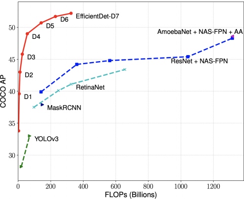
EfficientDet 是目前最优秀的检测器,backbone 是基于 depthwise separable convolution 和 SE 模块利用 AutoML 搜索出来的,EfficientDet 出彩的地方在于设计了高效的 FPN 结构,即 BiFPN。
摘要
模型的效率在计算机视觉中变得越发重要。本文系统地研究了神经网络结构在目标检测中的设计选择,并提出了提高检测效率的几个关键优化方案。首先,本文提出了一种加权的双向特征金字塔网络(BiFPN),它可以方便、快速地融合多尺度特征;其次,文中提出了一种混合缩放方法,可以同时对所有主干、特征网络和 box/class 预测网络的分辨率、深度和宽度进行均匀缩放。基于这些优化和 EfficientNet backbone, 文章开发了一类新的目标检测,称为 EfficientDet,该类检测算法比现有的检测算法都要高效。
以下部分为了图省事,参考的是 PyTorch 复现版本的代码,毕竟 TF1 调试不友好
以 d0 为例,计算量为:
backbone+fpn+box params/flops = 3.880067M, 2.535978423B
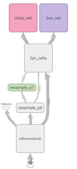
EfficientNet
检测网络的 backbone 采用的是 EfficientNet 系列,这一系列的网络是由 Auto ML 搜索出来的网络。网络的主要成分为 Depthwise Separable Conv 和 SENet 结构,这一系列网络结构从 B0 到 B7,有以下这些参数控制差别:
# Coefficients:   width,depth,res,dropout
'efficientnet-b0': (1.0, 1.0, 224, 0.2),
'efficientnet-b1': (1.0, 1.1, 240, 0.2),
'efficientnet-b2': (1.1, 1.2, 260, 0.3),
'efficientnet-b3': (1.2, 1.4, 300, 0.3),
'efficientnet-b4': (1.4, 1.8, 380, 0.4),
'efficientnet-b5': (1.6, 2.2, 456, 0.4),
'efficientnet-b6': (1.8, 2.6, 528, 0.5),
'efficientnet-b7': (2.0, 3.1, 600, 0.5)
1. 由 width 参数控制除 MBConvBlock 外两个卷积层(Stage1 和 Stage9)的输出通道数:


def round_filters(filters, global_params):
    """ Calculate and round number of filters based on depth multiplier. """
    multiplier = global_params.width_coefficient
    if not multiplier:
        return filters
    divisor = global_params.depth_divisor # default = 8
    min_depth = global_params.min_depth
    filters *= multiplier
    min_depth = min_depth or divisor       # min_depth default is None
    new_filters = max(min_depth, int(filters + divisor / 2) // divisor * divisor)
    if new_filters < 0.9 * filters:  # prevent rounding by more than 10%
        new_filters += divisor
    return int(new_filters)
2. 由 depth 控制 Block 重复次数(向上取整):
def round_repeats(repeats, global_params):
    """ Round number of filters based on depth multiplier. """
    multiplier = global_params.depth_coefficient
    if not multiplier:
        return repeats
    return int(math.ceil(multiplier * repeats))
3. res 控制图像输入尺度,dropout 控制最后 AVG_POOL 和 FC 之间的 DropOut 层的 dropout_rate
下面是基础的 EfficientNet-B0,MBConv 后面的数字代表深度可分离卷积中 expand 系数,Resolution 代表输入特征图分辨率, Channel 代表输出通道数,Layers 代表 Block 重复次数:
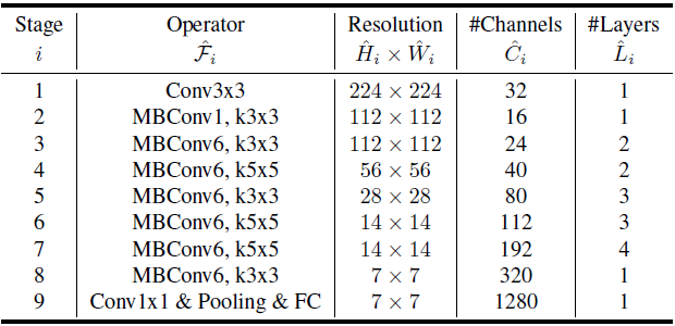 |
# Stem Stage1
x = self._swish(self._bn0(self._conv_stem(inputs)))

# Blocks Stage2-8
for idx, block in enumerate(self._blocks):
    drop_connect_rate = self._global_params.drop_connect_rate
    if drop_connect_rate:
        drop_connect_rate *= float(idx) / len(self._blocks)
    x = block(x, drop_connect_rate=drop_connect_rate)
# Head Stage9_1
x = self._swish(self._bn1(self._conv_head(x)))

# Pooling and final linear layer Stage9_2
x = self._avg_pooling(x)
x = x.view(bs, -1)
x = self._dropout(x)
x = self._fc(x)
|
默认每个深度可分离卷积中,DW 和 PW 之间会插入 SEblock, 同时默认开启 skip connection。
区别于常规的 CNNs, 如果 skip connection、stride=1 且 block 的输入和输出通道数相同则在 skip connection 之前、深度可分离卷积之后加上 dropout 操作!下面是 MBConvBlock 的部分实现:
# Expansion and Depthwise Convolution
x = inputs
if self._block_args.expand_ratio != 1:
    x = self._expand_conv(inputs)
    x = self._bn0(x)
    x = self._swish(x)

x = self._depthwise_conv(x)
x = self._bn1(x)
x = self._swish(x)

# Squeeze and Excitation
if self.has_se:
    x_squeezed = F.adaptive_avg_pool2d(x, 1)
    x_squeezed = self._se_reduce(x_squeezed)
    x_squeezed = self._swish(x_squeezed)
    x_squeezed = self._se_expand(x_squeezed)
    x = torch.sigmoid(x_squeezed) * x

x = self._project_conv(x)
x = self._bn2(x)

# Skip connection and drop connect
input_filters, output_filters = self._block_args.input_filters, self._block_args.output_filters
if self.id_skip and self._block_args.stride == 1 and input_filters == output_filters:
    if drop_connect_rate:
        x = drop_connect(x, p=drop_connect_rate, training=self.training)
    x = x + inputs  # skip connection
BiFPN
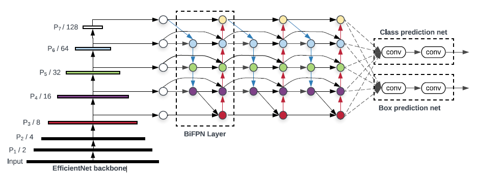
同 YOLOV3 等检测框架一样,EfficientDet 也加入了 FPN 元素来加强输出 feature map 的特征表示。区别在于 BiFPN 的连接更加复杂,同时可以作为一个基础层重复多次!
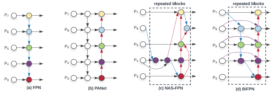
如上图所示:(a) 是传统的 FPN 结构,只有自顶向下的连接;(b) PANet 包括自顶向下和自底向上两条路径连接;(c) NAS-FPN 则是通过 NAS 搜出来的连连看结构。
作者观察到 PANet 的效果比 FPN 和 NAS-FPN 效果好,但就是计算量大了点。于是,作者从 PANet 出发,先移除掉了两个节点,然后在同一 level 的输入和输出节点之间,连上了一条线,有点 skip-connection 的味道。最后作者认为这样的连接可以作为一个基础 Block 而重复使用。
这里首先会将所有的输出 feature map 统一到相同 channel 来进行后续 Block 处理,这个 channel 数和 Block 重复次数也会根据不同的子版本而变化。
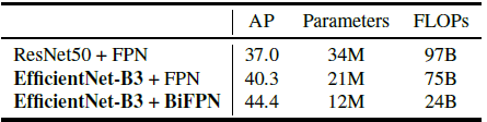
BiFPN 相比 FPN 能涨 4 个点,而且参数量反而是下降的:
Anchor
\begin{equation}
\label{Anchor}
\begin{split}
& anchor\_scale = 4.0 \\
& strides = [8, 16, 32, 64, 128] \\
& scales = [2^0, 2^{\frac{1}{3}}, 2^{\frac{2}{3}}] \\
& ratios = [(1.0, 1.0), (1.4, 0.7), (0.7, 1.4)] \\
& base\_anchor\_size = anchor\_scale * stride * scale \\
& anchor\_size\_w = base\_anchor_size * ratio[0] \\
& anchor\_size\_h = base\_anchor_size * ratio[1]
\end{split}
\end{equation}
每个尺度上共设计 9 个 Anchor,具体的,固定每个 feature map 上的 anchor _scale 为 4.0,将其映射到输出图片上并加入 scale 后就确定了 Anchor 的尺度 base_anchor_size 了。随后以每个大小的 Base Anchor 为基准,设计三种宽高比的 Anchor。
Regressor & Classifier
回归:每个预测的 feature map 会经过 N 次深度可分离卷积(DSC+BN+SW)后,再接上一个用于预测回归结果的深度可分离卷积(PW 的输出 channel = num_anchors * 4)。
分类:同上,区别只是最后的 PW 层输出 channel = num_anchors * num_classes。
Anchor+Regression
和 YOLOV3 编解码倒是很像,区别在于中心点偏移没有经过 sigmoid 函数:
记先验框($c_x, c_y, p_w, p_h$),其中 $c_x$ 和 $c_y$ 分别表示 Anchor 中心点距离图像左上角的距离,$p_w$ 和 $p_h$ 则分别表示先验框的宽和高。
记网络回归输出为($t_x, t_y, t_w, t_h$),其中$t_x$ 和 $t_y$ 用以偏移先验框的中心到检测框,$t_w$ 和 $t_h$ 则用来缩放先验框到检测框大小,
那么检测框($b_x, b_y, b_w, b_h$)可以用以下表达式表示:
\begin{equation}
\label{a}
\begin{split}
& b_x = t_x + c_x \\
& b_y = t_y + c_y \\
& b_w = p_w e^{t_w} \\
& b_h = p_h e^{t_h} \\
\end{split}
\end{equation}
LOSS
分类 loss 采用 focal loss,区别在于正负样本之间有个 margion,IoU < 0.4 的 Anchor 标记为负样本,IoU >= 0.5 的 Anchor 标记为正样本。
回归目标
\begin{equation}
\label{target}
\begin{split}
& \delta_x = (g_x - c_x) / p_w \\
& \delta_y = (g_y - c_y) / p_h \\
& \delta_w = log(g_w / p_w) \\
& \delta_h = log(g_h / p_h) \\
\end{split}
\end{equation}
回归 loss 则类似于 SmoothL1 loss:
\begin{equation}
\label{Smooth_L1}
smooth_{L_1}(x) = \begin{cases}
\ 0.5 * 9.0 * x^2 & if \ \lvert{x}\rvert < 1.0/9.0 \\
\ \lvert{x}\rvert - 0.5/9.0 & \ otherwise
\end{cases}
\end{equation}
Compound Scaling
Model Scaling 指的是人们经常根据资源的限制,对模型进行调整。比如说为了把 backbone 部分 scale up,得到更大的模型,就会考虑把层数加深, Res50 -> Res101这种,或者说比如把输入图的分辨率拉大。
EfficientNet 在 Model Scaling 的时候考虑了网络的 width, depth, and resolution 三要素。而 EfficientDet 进一步扩展, 把 EfficientNet 拿来做 backbone 的同时,neck 部分,BiFPN 的 channel 数量、重复的 layer 数量也可以控制;此外还有 head 部分的层数,以及 输入图片的分辨率,这些组成了 EfficientDet 的 scaling config 。
self.backbone_compound_coef = [0, 1, 2, 3, 4, 5, 6, 6]
self.fpn_num_filters = [64, 88, 112, 160, 224, 288, 384, 384]
self.fpn_cell_repeats = [3, 4, 5, 6, 7, 7, 8, 8]
self.input_sizes = [512, 640, 768, 896, 1024, 1280, 1280, 1536]
self.box_class_repeats = [3, 3, 3, 4, 4, 4, 5, 5]

 浙公网安备 33010602011771号