
深度学习笔记(十三)YOLO V3 (Tensorflow)
[原始代码]
[代码剖析] 推荐阅读!
之前看了一遍 YOLO V3 的论文,写的挺有意思的 ,尴尬的是,我这鱼的记忆,看完就忘了
于是只能借助于代码,再看一遍细节了。
源码目录总览
tensorflow-yolov3
    ├── checkpoint //保存模型的目录
    ├── convert_weight.py //对权重去冗余,去掉训练相关
    ├── core //核心代码文件夹
    │   ├── backbone.py
    │   ├── common.py
    │   ├── config.py //配置文件
    │   ├── dataset.py //数据处理
    │   ├── __init__.py
    │   ├── utils.py
    │   └── yolov3.py //网络核心结构
    ├── data
    │   ├── anchors // Anchor 配置
    │   │   ├── basline_anchors.txt
    │   │   └── coco_anchors.txt
    │   ├── classes //训练预测目标的种类
    │   │   ├── coco.names
    │   │   └── voc.names
    │   ├── dataset //保存图片的相关信息:路径,box,置信度,类别编号
    │   │   ├── voc_test.txt //测试数据
    │   │   └── voc_train.txt //训练数据
    ├── docs //比较混杂
    │   ├── Box-Clustering.ipynb //根据数据信息生成预选框anchors
    │   ├── images
    │   │   ├── 611_result.jpg
    │   │   ├── darknet53.png
    │   │   ├── iou.png
    │   │   ├── K-means.png
    │   │   ├── levio.jpeg
    │   │   ├── probability_extraction.png
    │   │   ├── road.jpeg
    │   │   ├── road.mp4
    │   │   └── yolov3.png
    │   └── requirements.txt // 环境需求
    ├── evaluate.py // 模型评估
    ├── freeze_graph.py //生成pb文件
    ├── image_demo.py // 利用 pb 模型的测试 demo
    ├── mAP//模型评估相关信息存储
    │   ├── extra
    │   │   ├── class_list.txt
    │   │   ├── convert_gt_xml.py
    │   │   ├── convert_gt_yolo.py
    │   │   ├── convert_keras-yolo3.py
    │   │   ├── convert_pred_darkflow_json.py
    │   │   ├── convert_pred_yolo.py
    │   │   ├── find_class.py
    │   │   ├── intersect-gt-and-pred.py
    │   │   ├── README.md
    │   │   ├── remove_class.py
    │   │   ├── remove_delimiter_char.py
    │   │   ├── remove_space.py
    │   │   ├── rename_class.py
    │   │   └── result.txt
    │   ├── __init__.py
    │   └── main.py // 计算 mAP
    ├── README.md
    ├── scripts
    │   ├── show_bboxes.py
    │   └── voc_annotation.py //把xml转化为网络可以使用的txt文件
    ├── train.py //模型训练
    └── video_demo.py // 利用 pb 模型的测试 demo
接下来,我按照看代码的顺序来详细说明了。
core/dataset.py


#! /usr/bin/env python
# coding=utf-8
# ================================================================
#   Copyright (C) 2019 * Ltd. All rights reserved.
#
#   Editor      : VIM
#   File name   : dataset.py
#   Author      : YunYang1994
#   Created date: 2019-03-15 18:05:03
#   Description :
#
# ================================================================

import os
import cv2
import random
import numpy as np
import tensorflow as tf
import core.utils as utils
from core.config import cfg


class DataSet(object):
    """implement Dataset here"""

    def __init__(self, dataset_type):
        self.annot_path = cfg.TRAIN.ANNOT_PATH if dataset_type == 'train' else cfg.TEST.ANNOT_PATH
        self.input_sizes = cfg.TRAIN.INPUT_SIZE if dataset_type == 'train' else cfg.TEST.INPUT_SIZE
        self.batch_size = cfg.TRAIN.BATCH_SIZE if dataset_type == 'train' else cfg.TEST.BATCH_SIZE
        self.data_aug = cfg.TRAIN.DATA_AUG if dataset_type == 'train' else cfg.TEST.DATA_AUG

        self.train_input_sizes = cfg.TRAIN.INPUT_SIZE
        self.strides = np.array(cfg.YOLO.STRIDES)
        self.classes = utils.read_class_names(cfg.YOLO.CLASSES)
        self.num_classes = len(self.classes)
        self.anchors = np.array(utils.get_anchors(cfg.YOLO.ANCHORS))
        self.anchor_per_scale = cfg.YOLO.ANCHOR_PER_SCALE
        self.max_bbox_per_scale = 150

        self.annotations = self.load_annotations(dataset_type)  # read and shuffle annotations
        self.num_samples = len(self.annotations)  # dataset size
        self.num_batchs = int(np.ceil(self.num_samples / self.batch_size))  # 向上取整
        self.batch_count = 0  # batch index

    def load_annotations(self, dataset_type):
        with open(self.annot_path, 'r') as f:
            txt = f.readlines()
            annotations = [line.strip() for line in txt if len(line.strip().split()[1:]) != 0]
        # np.random.seed(1)  # for debug
        np.random.shuffle(annotations)
        return annotations

    def __iter__(self):
        return self

    def next(self):
        with tf.device('/cpu:0'):
            self.train_input_size_h, self.train_input_size_w = random.choice(self.train_input_sizes)
            self.train_output_sizes_h = self.train_input_size_h // self.strides
            self.train_output_sizes_w = self.train_input_size_w // self.strides
            # ================================================================ #
            batch_image = np.zeros((self.batch_size, self.train_input_size_h, self.train_input_size_w, 3))

            batch_label_sbbox = np.zeros((self.batch_size, self.train_output_sizes_h[0], self.train_output_sizes_w[0],
                                          self.anchor_per_scale, 5 + self.num_classes))
            batch_label_mbbox = np.zeros((self.batch_size, self.train_output_sizes_h[1], self.train_output_sizes_w[1],
                                          self.anchor_per_scale, 5 + self.num_classes))
            batch_label_lbbox = np.zeros((self.batch_size, self.train_output_sizes_h[2], self.train_output_sizes_w[2],
                                          self.anchor_per_scale, 5 + self.num_classes))
            # ================================================================ #
            batch_sbboxes = np.zeros((self.batch_size, self.max_bbox_per_scale, 4))
            batch_mbboxes = np.zeros((self.batch_size, self.max_bbox_per_scale, 4))
            batch_lbboxes = np.zeros((self.batch_size, self.max_bbox_per_scale, 4))

            num = 0 # sample in one batch's index
            if self.batch_count < self.num_batchs:
                while num < self.batch_size:
                    index = self.batch_count * self.batch_size + num
                    if index >= self.num_samples:  # 从头开始
                        index -= self.num_samples
                    annotation = self.annotations[index]
                    # 样本预处理
                    image, bboxes = self.parse_annotation(annotation)
                    # Anchor & GT 匹配
                    label_sbbox, label_mbbox, label_lbbox, sbboxes, mbboxes, lbboxes = self.preprocess_true_boxes(
                        bboxes)

                    batch_image[num, :, :, :] = image
                    batch_label_sbbox[num, :, :, :, :] = label_sbbox
                    batch_label_mbbox[num, :, :, :, :] = label_mbbox
                    batch_label_lbbox[num, :, :, :, :] = label_lbbox
                    batch_sbboxes[num, :, :] = sbboxes
                    batch_mbboxes[num, :, :] = mbboxes
                    batch_lbboxes[num, :, :] = lbboxes
                    num += 1
                self.batch_count += 1
                return batch_image, batch_label_sbbox, batch_label_mbbox, batch_label_lbbox, \
                       batch_sbboxes, batch_mbboxes, batch_lbboxes
            else:
                self.batch_count = 0
                np.random.shuffle(self.annotations)
                raise StopIteration

    def random_horizontal_flip(self, image, bboxes):

        if random.random() < 0.5:
            _, w, _ = image.shape
            image = image[:, ::-1, :]
            bboxes[:, [0, 2]] = w - bboxes[:, [2, 0]]

        return image, bboxes

    def random_crop(self, image, bboxes):

        if random.random() < 0.5:
            h, w, _ = image.shape
            max_bbox = np.concatenate([np.min(bboxes[:, 0:2], axis=0), np.max(bboxes[:, 2:4], axis=0)], axis=-1)

            max_l_trans = max_bbox[0]
            max_u_trans = max_bbox[1]
            max_r_trans = w - max_bbox[2]
            max_d_trans = h - max_bbox[3]

            crop_xmin = max(0, int(max_bbox[0] - random.uniform(0, max_l_trans)))
            crop_ymin = max(0, int(max_bbox[1] - random.uniform(0, max_u_trans)))
            crop_xmax = max(w, int(max_bbox[2] + random.uniform(0, max_r_trans)))
            crop_ymax = max(h, int(max_bbox[3] + random.uniform(0, max_d_trans)))

            image = image[crop_ymin: crop_ymax, crop_xmin: crop_xmax]

            bboxes[:, [0, 2]] = bboxes[:, [0, 2]] - crop_xmin
            bboxes[:, [1, 3]] = bboxes[:, [1, 3]] - crop_ymin

        return image, bboxes

    def random_translate(self, image, bboxes):

        if random.random() < 0.5:
            h, w, _ = image.shape
            max_bbox = np.concatenate([np.min(bboxes[:, 0:2], axis=0), np.max(bboxes[:, 2:4], axis=0)], axis=-1)

            max_l_trans = max_bbox[0]
            max_u_trans = max_bbox[1]
            max_r_trans = w - max_bbox[2]
            max_d_trans = h - max_bbox[3]

            tx = random.uniform(-(max_l_trans - 1), (max_r_trans - 1))
            ty = random.uniform(-(max_u_trans - 1), (max_d_trans - 1))

            M = np.array([[1, 0, tx], [0, 1, ty]])
            image = cv2.warpAffine(image, M, (w, h))

            bboxes[:, [0, 2]] = bboxes[:, [0, 2]] + tx
            bboxes[:, [1, 3]] = bboxes[:, [1, 3]] + ty

        return image, bboxes

    def parse_annotation(self, annotation):

        line = annotation.split()
        image_path = line[0]
        if not os.path.exists(image_path):
            raise KeyError("%s does not exist ... " % image_path)
        image = np.array(cv2.imread(image_path))
        bboxes = np.array([list(map(int, box.split(','))) for box in line[1:]])

        if self.data_aug:
            image, bboxes = self.random_horizontal_flip(np.copy(image), np.copy(bboxes))
            image, bboxes = self.random_crop(np.copy(image), np.copy(bboxes))
            image, bboxes = self.random_translate(np.copy(image), np.copy(bboxes))

        image, bboxes = utils.image_preporcess(np.copy(image), [self.train_input_size_h, self.train_input_size_w],
                                               np.copy(bboxes))
        return image, bboxes

    def bbox_iou(self, boxes1, boxes2):

        boxes1 = np.array(boxes1)
        boxes2 = np.array(boxes2)

        boxes1_area = boxes1[..., 2] * boxes1[..., 3]
        boxes2_area = boxes2[..., 2] * boxes2[..., 3]

        boxes1 = np.concatenate([boxes1[..., :2] - boxes1[..., 2:] * 0.5,
                                 boxes1[..., :2] + boxes1[..., 2:] * 0.5], axis=-1)
        boxes2 = np.concatenate([boxes2[..., :2] - boxes2[..., 2:] * 0.5,
                                 boxes2[..., :2] + boxes2[..., 2:] * 0.5], axis=-1)

        left_up = np.maximum(boxes1[..., :2], boxes2[..., :2])
        right_down = np.minimum(boxes1[..., 2:], boxes2[..., 2:])

        inter_section = np.maximum(right_down - left_up, 0.0)
        inter_area = inter_section[..., 0] * inter_section[..., 1]
        union_area = boxes1_area + boxes2_area - inter_area

        return inter_area / union_area

    def preprocess_true_boxes(self, bboxes):
        # ================================================================ #
        label = [np.zeros((self.train_output_sizes_h[i], self.train_output_sizes_w[i], self.anchor_per_scale,
                           5 + self.num_classes)) for i in range(3)]
        """ match info
        hypothesis input size 320 x 480, label dim
        | 40 x 60 x 3 x 17 |
        | 20 x 30 x 3 x 17 |
        | 10 x 15 x 3 x 17 |
        """
        bboxes_xywh = [np.zeros((self.max_bbox_per_scale, 4)) for _ in range(3)]
        """ match gt set
        bboxes_xywh dim
        | 3 x 150 x 4 |
        """
        bbox_count = np.zeros((3,))
        # ================================================================ #
        for bbox in bboxes:
            bbox_coor = bbox[:4] # xmin, ymin, xmax, ymax
            bbox_class_ind = bbox[4] # class

            # smooth onehot label
            onehot = np.zeros(self.num_classes, dtype=np.float)
            onehot[bbox_class_ind] = 1.0
            uniform_distribution = np.full(self.num_classes, 1.0 / self.num_classes)
            deta = 0.01
            smooth_onehot = onehot * (1 - deta) + deta * uniform_distribution

            # box transform into 3 feature maps [center_x, center_y, w, h]
            bbox_xywh = np.concatenate([(bbox_coor[2:] + bbox_coor[:2]) * 0.5, bbox_coor[2:] - bbox_coor[:2]], axis=-1)
            bbox_xywh_scaled = 1.0 * bbox_xywh[np.newaxis, :] / self.strides[:, np.newaxis]

            # =========================== match iou ========================== #
            iou = [] # 3x3
            exist_positive = False
            for i in range(3): # different feature map
                anchors_xywh = np.zeros((self.anchor_per_scale, 4))
                anchors_xywh[:, 0:2] = np.floor(bbox_xywh_scaled[i, 0:2]).astype(np.int32) + 0.5
                anchors_xywh[:, 2:4] = self.anchors[i]

                iou_scale = self.bbox_iou(bbox_xywh_scaled[i][np.newaxis, :], anchors_xywh)
                iou.append(iou_scale)
                iou_mask = iou_scale > 0.3

                if np.any(iou_mask):
                    xind, yind = np.floor(bbox_xywh_scaled[i, 0:2]).astype(np.int32)

                    label[i][yind, xind, iou_mask, :] = 0
                    label[i][yind, xind, iou_mask, 0:4] = bbox_xywh
                    label[i][yind, xind, iou_mask, 4:5] = 1.0
                    label[i][yind, xind, iou_mask, 5:] = smooth_onehot

                    bbox_ind = int(bbox_count[i] % self.max_bbox_per_scale)
                    bboxes_xywh[i][bbox_ind, :4] = bbox_xywh
                    bbox_count[i] += 1

                    exist_positive = True

            if not exist_positive:
                best_anchor_ind = np.argmax(np.array(iou).reshape(-1), axis=-1)
                best_detect = int(float(best_anchor_ind) / self.anchor_per_scale)
                best_anchor = int(best_anchor_ind % self.anchor_per_scale)
                xind, yind = np.floor(bbox_xywh_scaled[best_detect, 0:2]).astype(np.int32)

                label[best_detect][yind, xind, best_anchor, :] = 0
                label[best_detect][yind, xind, best_anchor, 0:4] = bbox_xywh
                label[best_detect][yind, xind, best_anchor, 4:5] = 1.0
                label[best_detect][yind, xind, best_anchor, 5:] = smooth_onehot

                bbox_ind = int(bbox_count[best_detect] % self.max_bbox_per_scale)
                bboxes_xywh[best_detect][bbox_ind, :4] = bbox_xywh
                bbox_count[best_detect] += 1
        label_sbbox, label_mbbox, label_lbbox = label # different size feature map's anchor match info
        sbboxes, mbboxes, lbboxes = bboxes_xywh       # different size feature map's matched gt set
        return label_sbbox, label_mbbox, label_lbbox, sbboxes, mbboxes, lbboxes

    def __len__(self):
        return self.num_batchs


if __name__ == '__main__':
    val = DataSet('test')
    for idx in range(val.num_batchs):
        batch_image, batch_label_sbbox, batch_label_mbbox, batch_label_lbbox, \
        batch_sbboxes, batch_mbboxes, batch_lbboxes = val.next()
    print('# ================================================================ #')
这部分是用来加载数据的。
整个 core/dataset.py 实现了一个 DataSet 类,每个 batch 的数据通过迭代函数 next() 获得。
self.trainset = DataSet('train')
pbar = tqdm(self.trainset)
for train_data in pbar:
    ....
    pbar.set_description(("train loss: %.2f" "learn rate: %e") % (train_step_loss, learn_rate))

for test_data in self.testset:
    ....
函数返回
batch_image       # one batch resized images
batch_label_sbbox # 第一个尺度下的匹配结果
batch_label_mbbox # 第二个尺度下的匹配结果
batch_label_lbbox # 第三个尺度下的匹配结果
batch_sbboxes     # 第一个尺度下匹配的 GT 集合
batch_mbboxes     # 第二个尺度下匹配的 GT 集合
batch_lbboxes     # 第三个尺度下匹配的 GT 集合
其中 batch_image 为网络输入特征,按照 NxHxWxC 维度排列,batch_label_sbbox、batch_label_mbbox 、batch_label_lbbox 这三个用以确定不同尺度下的 anchor 做正样本还是负样本;batch_sbboxes、batch_mbboxes、batch_lbboxes 这三个就有点意思了,是为了后续区分负样本是否有可能变成正样本(回归到 bbox 了) 做准备。
,可以继续往下看。数据集在 DataSet 初始化的时候就被打乱了,如果你想每次调试运行看看上面的代码是怎么工作的,可以再 load_annotations() 函数里固定随机因子
np.random.seed(1)
数据格式
不管你训练什么数据集(VOC、COCO),数据的标注格式都要转换成以下格式 ' image_path [bbox class] ...':
D:/tyang/drive0703/JPEGImages/test_dataset_without2018/2017_07_24_10_49_026073.jpg 466,396,582,475,0 289,394,377,449,0 689,432,788,504,0 778,435,839,481,0 856,433,887,458,2 612,419,653,446,3
当然,scripts/voc_annotation.py 提供了将 VOC 的 xml 格式转换成需求格式,这部分不是很难,其他格式的数据集,自己瞎写写转一转也没啥问题。
数据预处理
对于每个样本,先经过预处理函数 parse_annotation() 加载 image & bboxes,对于训练数据,这里会执行一些 data argument。
假定不做 data argument,bboxes 就只是变成了缩放后的图片下的框坐标值

Anchor & GT 匹配
然后,最重要的部分来了,通过 preprocess_true_boxes() 来实现 Anchor & GT 匹配:
label = [np.zeros((self.train_output_sizes_h[i], self.train_output_sizes_w[i], self.anchor_per_scale,
                           5 + self.num_classes)) for i in range(3)]
""" match info
hypothesis input size 320 x 480 with 12 classes, label dim
| 40 x 60 x 3 x 17 | # label_sbbox
| 20 x 30 x 3 x 17 | # label_mbbox
| 10 x 15 x 3 x 17 | # label_lbbox
"""
bboxes_xywh = [np.zeros((self.max_bbox_per_scale, 4)) for _ in range(3)]
""" match gt set
bboxes_xywh dim
| 3 x 150 x 4 |      # sbboxes, mbboxes, lbboxes
"""
label 里保存的是三个尺度下的 Anchor 的匹配情况;bboxes_xywh 里则保存的是三个尺度小被匹配上的 GT 集合。
网络在三个尺度的 feature map 下检测目标,这三个尺度的 feature map 由输入图片分别经过 stride=8, 16, 32 获得。
假定训练中输入尺度是 320x480,那么这三个 feature map size: 40x60, 20x30, 10x15。
对于每个 feature map 下,作者分别设计(聚类)了三种 anchor,例如 data/anchors/basline_anchors.txt 中:
# small
1.25,1.625
2.0,3.75
4.125,2.875
# middle
1.875,3.8125
3.875,2.8125
3.6875,7.4375
# large
3.625,2.8125
4.875,6.1875
11.65625,10.1875
因此,第一个尺度里有 40 x 60 x 3 = 7200 个 anchor;第二个尺度里有 20 x 30 x 3 = 1800 个 anchor;第三个尺度里有 10x 15x 3 = 450 个 anchor。
值得注意的是,原始 bbox 是按照 [xmin, ymin, xmax, ymax],需要转换成 [center_x, center_y, w, h] 被保存在匹配结果里,即:
[116 117 145 140] -> [130.5 128.5 29. 23. ]
[ 72 116 94 133] -> [ 83. 124.5 22. 17. ]
[172 128 197 149] -> [184.5 138.5 25. 21. ]
[194 128 209 142] -> [201.5 135. 15. 14. ]
[214 128 221 135] -> [217.5 131.5 7. 7. ]
[153 124 163 132] -> [158. 128. 10. 8. ]
label 最后一个维度是 5 + self.num_classes,其中 5, 前 4 维是 [center_x, center_y, w, h] GT bbox, 第 5 维是 0/1, 0 表示无匹配,1 表示匹配成功。self.num_classes 用来表示目标类别,之所以要用这么多维数据来表示,是因为将整形 label 转换成了 one-hot 形式。同时这里做了 label smooth 操作,例如 label 0 ->[9.90833333e-01 8.33333333e-04 8.33333333e-04 8.33333333e-04 8.33333333e-04 8.33333333e-04 8.33333333e-04 8.33333333e-04 8.33333333e-04 8.33333333e-04 8.33333333e-04 8.33333333e-04]。
# smooth onehot label
onehot = np.zeros(self.num_classes, dtype=np.float)
onehot[bbox_class_ind] = 1.0
uniform_distribution = np.full(self.num_classes, 1.0 / self.num_classes)
deta = 0.01
smooth_onehot = onehot * (1 - deta) + deta * uniform_distribution
每个 GT bbox 会和三个尺度上所在位置处所有的 anchor 尝试匹配 match anchor,并将匹配结果保存作为网络训练输入的一部分。对于每个 bbox(下面会以 [130.5 128.5 29. 23. ] 这个 bbox 为例):
- 将 bbox 映射到每个 feature map 上,获得 bbox_xywh_scaled :
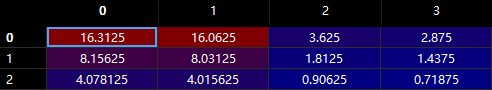
- 在每个尺度上尝试匹配,为了计算效率,只利用中心的在 bbox 中心点的 anchor 尝试匹配,例如第一个尺度上的 bbox=[16.3125 16.0625 3.625 2.875 ] 将尝试与 small anchor 集合(anchors_xywh) 进行匹配:
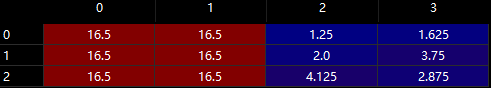
- 匹配计算 bbox_iou -> [0.19490255 0.47240051 0.65717606],如果找到满足大于 0.3 的一对,即为匹配成功 (False, True, True)。匹配成功后就往 label 和 bboxes_xywh 里填信息就好了。
"""
label[1][16, 16, [False  True  True], :] = 0
label[1][16, 16, [False  True  True], 0:4] = bbox_xywh #[130.5  128.5  29.  23.]
label[1][16, 16, [False  True  True], 4:5] = 1.0
label[1][16, 16, [False  True  True], 5:] = smooth_obehot
bboxes_xywh[1][bbox_ind, :4] = bbox_xywh #[130.5  128.5  29.   23. ]
""" bbox_ind 是这个尺度下累计匹配成功的 GT 数量,代码中限制范围 [0-149]
- 如果有 bbox 在各个 feature map 都找不到满足的匹配 anchor,那就退而求其次,在所有三个尺度下的 anchor(9个) 里寻找一个最大匹配就好了。
到此,匹配结束。
train.py
INPUT
输入层对应 dataset.py 每个batch 返回的变量
with tf.name_scope('define_input'):
    self.input_data = tf.placeholder(dtype=tf.float32, name='input_data', shape=[None, None, None, 3])
    self.label_sbbox = tf.placeholder(dtype=tf.float32, name='label_sbbox')
    self.label_mbbox = tf.placeholder(dtype=tf.float32, name='label_mbbox')
    self.label_lbbox = tf.placeholder(dtype=tf.float32, name='label_lbbox')
    self.true_sbboxes = tf.placeholder(dtype=tf.float32, name='sbboxes')
    self.true_mbboxes = tf.placeholder(dtype=tf.float32, name='mbboxes')
    self.true_lbboxes = tf.placeholder(dtype=tf.float32, name='lbboxes')
    self.trainable = tf.placeholder(dtype=tf.bool, name='training')
MODEL & LOSS
YOLOV3 的 loss 分为三部分,回归 loss, 二分类(前景/背景) loss, 类别分类 loss
with tf.name_scope("define_loss"):
    self.model = YOLOV3(self.input_data, self.trainable, self.net_flag)
    self.net_var = tf.global_variables()
    self.giou_loss, self.conf_loss, self.prob_loss = self.model.compute_loss(self.label_sbbox,
                                                                             self.label_mbbox,
                                                                             self.label_lbbox,
                                                                             self.true_sbboxes,
                                                                             self.true_mbboxes,
                                                                             self.true_lbboxes)
    self.loss = self.giou_loss + self.conf_loss + self.prob_loss
Learning rate
with tf.name_scope('learn_rate'):
    self.global_step = tf.Variable(1.0, dtype=tf.float64, trainable=False, name='global_step')
    warmup_steps = tf.constant(self.warmup_periods * self.steps_per_period,
                               dtype=tf.float64, name='warmup_steps') # warmup_periods epochs
    train_steps = tf.constant((self.first_stage_epochs + self.second_stage_epochs) * self.steps_per_period,
                              dtype=tf.float64, name='train_steps')
    self.learn_rate = tf.cond(
        pred=self.global_step < warmup_steps,
        true_fn=lambda: self.global_step / warmup_steps * self.learn_rate_init,
        false_fn=lambda: self.learn_rate_end + 0.5 * (self.learn_rate_init - self.learn_rate_end) * (
                    1 + tf.cos((self.global_step - warmup_steps) / (train_steps - warmup_steps) * np.pi)))
    global_step_update = tf.assign_add(self.global_step, 1.0)
    """
    训练分为两个阶段,第一阶段里前面又划分出一段作为“热身阶段”:
    热身阶段:learn_rate = (global_step / warmup_steps) * learn_rate_init
    其他阶段:learn_rate_end + 0.5 * (learn_rate_init - learn_rate_end) * (
                    1 + tf.cos((global_step - warmup_steps) / (train_steps - warmup_steps) * np.pi))
    """
假定遍历一遍数据集需要 100 batch, warmup_periods=2, first_stage_epochs=20, second_stage_epochs=30, learn_rate_init=1e-4, learn_rate_end=1e-6, 那么整个训练过程中学习率是这样的:
import numpy as np
import matplotlib.pyplot as plt

steps_per_period = 100
warmup_periods=2
first_stage_epochs=20
second_stage_epochs=30
learn_rate_init=1e-4
learn_rate_end=1e-6
warmup_steps = warmup_periods * steps_per_period
train_steps = (first_stage_epochs + second_stage_epochs) * steps_per_period

def learn_rate_strategy(global_step, warmup_steps, train_steps,
                        learn_rate_init, learn_rate_end):
    """

    :param global_step:
    :param warmup_steps:
    :param learn_rate_init:
    :param learn_rate_end:
    :return:
    """
    if global_step < warmup_steps:
        learn_rate = (global_step / warmup_steps) * learn_rate_init
    else:
        learn_rate = learn_rate_end + 0.5 * (learn_rate_init - learn_rate_end) * (
                            1 + np.cos((global_step - warmup_steps) / (train_steps - warmup_steps) * np.pi))
    return learn_rate

learn_rate_list = []

for step in range(train_steps):
    learing_rate = learn_rate_strategy(step, warmup_steps, train_steps,
                        learn_rate_init, learn_rate_end)
    learn_rate_list.append(learing_rate)

step = range(train_steps)

print(learn_rate_list[-1])

plt.plot(step, learn_rate_list, 'g-', linewidth=2, label='learing_rate')
plt.xlabel('step')
plt.ylabel('learing rate')
plt.legend(loc='upper right')
plt.tight_layout()
plt.show()

two stage train
整个训练按照任务划分成了两个阶段,之所以这么设计,是考虑作者是拿原始的 DarkNet 来 finetune 的。
finetune 的一般流程就是,利用预训练的模型赋初值,先固定 backbone,只训练最后的分类/回归层。然后放开全部训练。
也可以对于浅层特征可以用小的学习率来微调(因为网络里浅层特征提取的边界纹理信息可能都是相近的,不需要作大调整),越接近于输出层可能需要调整的越多,输出层因为没有用其他模型初始化(随机初始化),因此需要从头训练。
for epoch in range(1, 1 + self.first_stage_epochs + self.second_stage_epochs):
    if epoch <= self.first_stage_epochs:
        train_op = self.train_op_with_frozen_variables
    else:
        train_op = self.train_op_with_all_variables
first_stage_train
这个阶段将专注于训练最后的检测部分,即分类和回归
with tf.name_scope("define_first_stage_train"):
    self.first_stage_trainable_var_list = []
    for var in tf.trainable_variables():
        var_name = var.op.name
        var_name_mess = str(var_name).split('/')
        if var_name_mess[0] in ['conv_sbbox', 'conv_mbbox', 'conv_lbbox']:
            self.first_stage_trainable_var_list.append(var)

    first_stage_optimizer = tf.train.AdamOptimizer(self.learn_rate).minimize(self.loss,
                                                                             var_list=self.first_stage_trainable_var_list)
    with tf.control_dependencies(tf.get_collection(tf.GraphKeys.UPDATE_OPS)):
        with tf.control_dependencies([first_stage_optimizer, global_step_update]):
            with tf.control_dependencies([moving_ave]):
                self.train_op_with_frozen_variables = tf.no_op()
second_stage_train
这个阶段就是整体训练,没什么好说的
with tf.name_scope("define_second_stage_train"):
    second_stage_trainable_var_list = tf.trainable_variables()
    second_stage_optimizer = tf.train.AdamOptimizer(self.learn_rate).minimize(self.loss,
                                                                              var_list=second_stage_trainable_var_list)

    with tf.control_dependencies(tf.get_collection(tf.GraphKeys.UPDATE_OPS)):
        with tf.control_dependencies([second_stage_optimizer, global_step_update]):
            with tf.control_dependencies([moving_ave]):
                self.train_op_with_all_variables = tf.no_op()
ExponentialMovingAverage
with tf.name_scope("define_weight_decay"):
    moving_ave = tf.train.ExponentialMovingAverage(self.moving_ave_decay).apply(tf.trainable_variables())
这个我涉世未深,还不甚明了,参见 tf.train.ExponentialMovingAverage
core/backbone.py
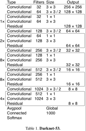
这里定义了 Darknet-53 的主题框架
| 网络结构 | 代码结构 |
|---|---|
 |
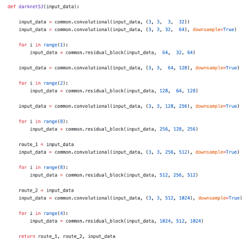 |
当然,你也可以根据你的需要,定义一些其他的 backbone,例如 mobilenet_v2。
core/yolov3.py
这里是整个 YOLOV3 代码的灵魂之处了。
__build_nework
YOLOV3 同 SSD 一样,是多尺度目标检测。选择了 stride=8, 16, 32 三个尺度的 feature map 来设计 anchor, 以便分别实现对小、中和大物体的预测。
假定输入尺度是 320x480,那么这三个 feature map 的大小就是 40x60, 20x30, 10x15。分别在这三个尺度的 feature map 的基础上,通过 3*(4+1+classes) 个 3x3 的卷积核卷积来预测分类和回归结果。这里 3 代表每个尺度下设计了 3 中不同尺寸的 anchor,4 是 bbox 回归预测,1 则是表示该 anchor 是否包含目标,classes 则是你的数据集里具体的类别数量了。如此,可以推测出每个尺度下的预测输出维度为(我的数据集包含 12 个类别目标):
batch_size x 40 x 60 x 51
batch_size x 20 x 30 x 51
batch_size x 10 x 15 x 51
这些预测输出将和 core/dataset.py 文件里获得的 GT 信息作比较,计算 loss。
upsample
网络在 backbone 特征提取的基础上加上了上采样特征连接,加强了浅层特征表示。
def upsample(input_data, name, method="deconv"):
    assert method in ["resize", "deconv"]

    if method == "resize":
        with tf.variable_scope(name):
            input_shape = tf.shape(input_data)
            output = tf.image.resize_nearest_neighbor(input_data, (input_shape[1] * 2, input_shape[2] * 2))

    if method == "deconv":
        # replace resize_nearest_neighbor with conv2d_transpose To support TensorRT optimization
        numm_filter = input_data.shape.as_list()[-1]
        output = tf.layers.conv2d_transpose(input_data, numm_filter, kernel_size=2, padding='same',
                                            strides=(2, 2), kernel_initializer=tf.random_normal_initializer())
这里提供了两种实现方式,最近邻缩放和反卷积。
decode
同 SSD 类似,anchor 的回归并非直接坐标回归,而是通过编码后进行回归:

我们知道,检测框实际上是在先验框的基础上回归出来的。如上图所示:在其中一个输出尺度下的 feature map 上,有一个黑色的先验框($c_x, c_y, p_w, p_h$),其中 $c_x$ 和 $c_y$ 分别表示中心网格距离图像左上角的距离,$p_w$ 和 $p_h$ 则分别表示先验框的宽和高。
记网络回归输出为($t_x, t_y, t_w, t_h$),其中$t_x$ 和 $t_y$ 用以偏移先验框的中心到检测框,$t_w$ 和 $t_h$ 则用来缩放先验框到检测框大小,那么蓝色的检测框($b_x, b_y, b_w, b_h$)可以用以下表达式表示:
\begin{equation}
\label{a}
\begin{split}
& b_x = \sigma(t_x) + c_x \\
& b_y = \sigma(t_y) + c_y \\
& b_w = p_w e^{t_w} \\
& b_h = p_h e^{t_h} \\
\end{split}
\end{equation}
具体实现:
def decode(self, conv_output, anchors, stride):
    """
    return tensor of shape [batch_size, output_size, output_size, anchor_per_scale, 5 + num_classes]
           contains (x, y, w, h, score, probability)
    """

    conv_shape = tf.shape(conv_output)
    batch_size = conv_shape[0]
    output_size_h = conv_shape[1]
    output_size_w = conv_shape[2]
    anchor_per_scale = len(anchors)

    conv_output = tf.reshape(conv_output,
                             (batch_size, output_size_h, output_size_w, anchor_per_scale, 5 + self.num_class))

    conv_raw_dxdy = conv_output[:, :, :, :, 0:2]
    conv_raw_dwdh = conv_output[:, :, :, :, 2:4]
    conv_raw_conf = conv_output[:, :, :, :, 4:5]
    conv_raw_prob = conv_output[:, :, :, :, 5:]

    # 划分网格
    y = tf.tile(tf.range(output_size_h, dtype=tf.int32)[:, tf.newaxis], [1, output_size_w])
    x = tf.tile(tf.range(output_size_w, dtype=tf.int32)[tf.newaxis, :], [output_size_h, 1])

    xy_grid = tf.concat([x[:, :, tf.newaxis], y[:, :, tf.newaxis]], axis=-1)
    xy_grid = tf.tile(xy_grid[tf.newaxis, :, :, tf.newaxis, :], [batch_size, 1, 1, anchor_per_scale, 1])
    xy_grid = tf.cast(xy_grid, tf.float32) # 计算网格左上角的位置

    # 根据论文公式计算预测框的中心位置
    pred_xy = (tf.sigmoid(conv_raw_dxdy) + xy_grid) * stride
    # 根据论文公式计算预测框的长和宽大小
    pred_wh = (tf.exp(conv_raw_dwdh) * anchors) * stride
    # 合并边界框的位置和长宽信息
    pred_xywh = tf.concat([pred_xy, pred_wh], axis=-1)

    pred_conf = tf.sigmoid(conv_raw_conf) # 计算预测框里object的置信度
    pred_prob = tf.sigmoid(conv_raw_prob) # 计算预测框里object的类别概率

    return tf.concat([pred_xywh, pred_conf, pred_prob], axis=-1)
compute_loss & loss_layer
代码分别从三个尺度出发,分别计算 边界框损失(giou_loss)、是否包含目标的置信度损失(conf_loss)以及具体类别的分类损失(prob_loss)
def compute_loss(self, label_sbbox, label_mbbox, label_lbbox, true_sbbox, true_mbbox, true_lbbox):

    with tf.name_scope('smaller_box_loss'):
        loss_sbbox = self.loss_layer(self.conv_sbbox, self.pred_sbbox, label_sbbox, true_sbbox,
                                     anchors=self.anchors[0], stride=self.strides[0])

    with tf.name_scope('medium_box_loss'):
        loss_mbbox = self.loss_layer(self.conv_mbbox, self.pred_mbbox, label_mbbox, true_mbbox,
                                     anchors=self.anchors[1], stride=self.strides[1])

    with tf.name_scope('bigger_box_loss'):
        loss_lbbox = self.loss_layer(self.conv_lbbox, self.pred_lbbox, label_lbbox, true_lbbox,
                                     anchors=self.anchors[2], stride=self.strides[2])

    with tf.name_scope('giou_loss'):
        giou_loss = loss_sbbox[0] + loss_mbbox[0] + loss_lbbox[0]

    with tf.name_scope('conf_loss'):
        conf_loss = loss_sbbox[1] + loss_mbbox[1] + loss_lbbox[1]

    with tf.name_scope('prob_loss'):
        prob_loss = loss_sbbox[2] + loss_mbbox[2] + loss_lbbox[2]

    return giou_loss, conf_loss, prob_loss
GIoU Loss
同 SSD(smooth L1 loss) 等检测算法相比,这里使用 GIoU 来衡量检测框和 GT bbox 之间的差距,具体可以参考论文和本代码作者的解读。

giou = tf.expand_dims(self.bbox_giou(pred_xywh, label_xywh), axis=-1)
input_size_w = tf.cast(input_size_w, tf.float32)
input_size_h = tf.cast(input_size_h, tf.float32)
# giou_loss 权重, [1, 2], 增加小目标的回归权重
bbox_loss_scale = 2.0 - 1.0 * label_xywh[:, :, :, :, 2:3] * label_xywh[:, :, :, :, 3:4] / (
        input_size_w * input_size_h)
# 所有匹配框计算回归 loss, 未匹配的 anchor 计算出来的 giou 值是无效值,因为 label_xywh 为 0
giou_loss = respond_bbox * bbox_loss_scale * (1 - giou) # giou_loss = (2 - bbox_area/image_area) * (1 - giou)
Focal Loss
网格中的 anchor 是否包含目标,这是个逻辑回归问题。作者这里引入了 Focal Loss,给纯背景框的 loss 进行压缩,Focal loss 的作用可参考论文。
iou = self.bbox_iou(pred_xywh[:, :, :, :, np.newaxis, :], bboxes[:, np.newaxis, np.newaxis, np.newaxis, :, :])
# 找出与真实框 iou 值最大的预测框(3 种 anchor 回归后取 1,匹配最好的Anchor经过回归后不一定是与 bbox iou 最高)
max_iou = tf.expand_dims(tf.reduce_max(iou, axis=-1), axis=-1)
# 匹配阶段和回归后均为负样本的纯背景 anchor (意味着匹配阶段为负样本,回归性能却不错的 Anchor 被 conf_loss 忽略)
respond_bgd = (1.0 - respond_bbox) * tf.cast(max_iou < self.iou_loss_thresh, tf.float32)
# 计算 loss 权重,给予分错检测框 loss 更多的惩罚
conf_focal = self.focal(respond_bbox, pred_conf)
# 计算置信度的损失
conf_loss = conf_focal * (
        # 匹配阶段为正样本的 anchor 分类 loss
        respond_bbox * tf.nn.sigmoid_cross_entropy_with_logits(labels=respond_bbox, logits=conv_raw_conf)
        +
        # 纯背景 anchor 分类 loss
        respond_bgd * tf.nn.sigmoid_cross_entropy_with_logits(labels=respond_bbox, logits=conv_raw_conf)
) # 这里对匹配阶段为负样本, 经过回归后和 bbox 的 iou > 0.5 的 anchor, 不计算分类 loss
分类损失
最后这个分类损失就没什么好说的了,采用的是二分类的交叉熵,即把所有类别的分类问题归结为是否属于这个类别,这样就把多分类看做是二分类问题。
prob_loss = respond_bbox * tf.nn.sigmoid_cross_entropy_with_logits(labels=label_prob, logits=conv_raw_prob)
K-means
先验框的设计一直是个比较头疼的问题,我在 SSD 里设计的 anchor 基本上是基于数据集的目标分布来人工设计出来的,这种设计比一定合适,而且很麻烦。
YOLOV3 里就比较偷懒了,他也是根据数据集分布来设计的,只不过人家更高级,用聚类来自动实现。
we run k-means clustering on the training set bounding boxes to automatically find good priors.
即使用 k-means 算法对训练集上的 boudnding box 尺度做聚类。此外,考虑到训练集上的图片尺寸不一,因此对此过程进行归一化处理。
k-means 聚类算法有个坑爹的地方在于,类别的个数需要事先指定。这就带来一个问题,先验框 anchor 的数目等于多少最合适?一般来说,anchor 的类别越多,那么 YOLO 算法就越能在不同尺度下与真实框进行回归,但是这样就导致模型的复杂度更高,网络的参数量更庞大。

We choose k = 5 as a good tradeoff between model complexity and high recall. If we use 9 centroids we see a much higher average IOU. This indicates that using k-means to generate our bounding box starts the model off with a better representation and makes the task easier to learn.
在上面这张图里,作者发现 k=5 时就能较好的实现高召回率和模型复杂度之间的平衡。由于在 YOLOV3 算法里一种有 3 个尺度预测,因此只能是 3 的倍数,所以最终选择了 9 个先验框。这里还有个问题需要解决,k-means 度量距离的选取很关键。距离度量如果使用标准的欧氏距离,大框框就会比小框产生更多的错误。在目标检测领域,我们度量两个边界框之间的相似度往往以 IOU 大小作为标准。因此,这里的度量距离也和 IOU 有关。需要特别注意的是,这里的IOU计算只用到了 boudnding box 的长和宽。在作者的代码里,是认为两个先验框的左上角位置是相重合的。(其实在这里偏移至哪都无所谓,因为聚类的时候是不考虑 anchor 框的位置信息的。)
\begin{equation}
\label{b}
d(box, centroid) = 1 - IOU(box, centroid)
\end{equation}
如果两个边界框之间的IOU值越大,那么它们之间的距离就会越小。
def kmeans(boxes, k, dist=np.median,seed=1):
    """
    Calculates k-means clustering with the Intersection over Union (IoU) metric.
    :param boxes: numpy array of shape (r, 2), where r is the number of rows
    :param k: number of clusters
    :param dist: distance function
    :return: numpy array of shape (k, 2)
    """
    rows = boxes.shape[0]

    distances     = np.empty((rows, k)) ## N row x N cluster
    last_clusters = np.zeros((rows,))

    np.random.seed(seed)

    # initialize the cluster centers to be k items
    clusters = boxes[np.random.choice(rows, k, replace=False)]

    while True:
        # 为每个点指定聚类的类别(如果这个点距离某类别最近,那么就指定它是这个类别)
        for icluster in range(k): # I made change to lars76's code here to make the code faster
            distances[:,icluster] = 1 - iou(clusters[icluster], boxes)

        nearest_clusters = np.argmin(distances, axis=1)
    # 如果聚类簇的中心位置基本不变了,那么迭代终止。
        if (last_clusters == nearest_clusters).all():
            break

        # 重新计算每个聚类簇的平均中心位置,并它作为聚类中心点
        for cluster in range(k):
            clusters[cluster] = dist(boxes[nearest_clusters == cluster], axis=0)

        last_clusters = nearest_clusters

    return clusters,nearest_clusters,distances
NMS 处理
熟悉检测的人一般都了解非极大值抑制(Non-Maximum Suppression,NMS)这一过程。直白的理解就是去除掉那些重叠率较高并且 score 评分较低的检测框。
NMS 的算法非常简单,迭代流程如下:
- 流程1:判断检测框的数目是否大于0,如果不是则结束迭代;
- 流程2:按照 score 排序选出评分最大的检测框 A 并取出;
- 流程3:计算这个边界框 A 与剩下所有检测框的 iou 并剔除那些 iou 值高于阈值的其他检测框,重复上述步骤
while len(cls_bboxes) > 0:
    max_ind = np.argmax(cls_bboxes[:, 4])
    best_bbox = cls_bboxes[max_ind]
    best_bboxes.append(best_bbox)
    cls_bboxes = np.concatenate([cls_bboxes[: max_ind], cls_bboxes[max_ind + 1:]])
    iou = bboxes_iou(best_bbox[np.newaxis, :4], cls_bboxes[:, :4])
    weight = np.ones((len(iou),), dtype=np.float32)

    assert method in ['nms', 'soft-nms']

    if method == 'nms':
        iou_mask = iou > iou_threshold
        weight[iou_mask] = 0.0

    if method == 'soft-nms':
        weight = np.exp(-(1.0 * iou ** 2 / sigma))

    cls_bboxes[:, 4] = cls_bboxes[:, 4] * weight
    score_mask = cls_bboxes[:, 4] > 0.
    cls_bboxes = cls_bboxes[score_mask]
在 YOLO 算法中,NMS 的处理有两种情况:一种是所有的预测框一起做 NMS 处理,另一种情况是分别对每个类别的预测框做 NMS 处理。后者会出现一个预测框既属于类别 A 又属于类别 B 的现象,这比较适合于一个小单元格中同时存在多个物体的情况。
evaluate.py
该代码输出包括三部分:
1. 每张图片的检测结果(文件名按从0开始的序号表示了,mAP/predicted/)
# class score xmin ymin xmax ymax
car 0.9625 680 425 780 504
car 0.9160 470 397 591 471
car 0.9015 775 434 840 489
car 0.4170 293 392 370 429
bus 0.4381 844 433 887 468
van 0.4556 613 411 653 444
2. 每张图片的GT(mAP/ground-truth/)
# class xmin ymin xmax ymax
car 466 396 582 475
car 289 394 377 449
car 689 432 788 504
car 778 435 839 481
bus 856 433 887 458
van 612 419 653 446
3. 每张图片可视化检测结果(self.write_image_path)
mAP/main.py
这部分就是利用上一步得到的 GT 和检测结果来计算 mAP 的过程了。
搬运源作者的训练技巧
1. Xavier initialization
2. 学习率的设置
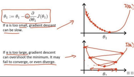
学习率是最影响性能的超参数之一,如果我们只能调整一个超参数,那么最好的选择就是它。 其实在我们的大多数的炼丹过程中,遇到 loss 变成 NaN 的情况大多数是由于学习率选择不当引起的。有句话讲得好啊,步子大了容易扯到蛋。由于神经网络在刚开始训练的时候是非常不稳定的,因此刚开始的学习率应当设置得很低很低,这样可以保证网络能够具有良好的收敛性。但是较低的学习率会使得训练过程变得非常缓慢,因此这里会采用以较低学习率逐渐增大至较高学习率的方式实现网络训练的“热身”阶段,称为 warmup stage。但是如果我们使得网络训练的 loss 最小,那么一直使用较高学习率是不合适的,因为它会使得权重的梯度一直来回震荡,很难使训练的损失值达到全局最低谷。因此最后采用了这篇论文里的 cosine 的衰减方式,这个阶段可以称为 consine decay stage。
3. 加载预训练模型
其实加载预训练模型,也是避免梯度溢出的一种有效方式。
目前针对目标检测的主流做法是基于 Imagenet 数据集预训练的模型来提取特征,然后在 COCO 数据集进行目标检测fine-tunning训练(比如 yolo 算法),也就是大家常说的迁移学习。其实迁移学习是建立在数据集分布相似的基础上的,像 yymnist 这种与 COCO 数据集分布完全不同的情况,就没有必要加载 COCO 预训练模型的必要了吧。
在 tensorflow-yolov3 版本里,由于 README 里训练的是 VOC 数据集,因此推荐加载预训练模型。由于在 YOLOv3 网络的三个分支里的最后卷积层与训练的类别数目有关,因此除掉这三层的网络权重以外,其余所有的网络权重都加载进来了。
我加载的是作者已经训练好的网络,因此可以这么干。但事实上作者是利用 darknet53 网络在 Imagenet 数据集上进行分类训练得到 darknet53.conv.74 权重后,再加载至 YOLOv3 网络里进行目标检测训练的!
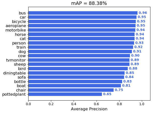
作者在 PASCAL VOC 2012 上比赛刷到了 88.38% 的成绩
Convert to PB
1. 调用 convert_weight.py 去掉 ckpt 模型中有关训练的冗余参数,比较转换前后的模型,你会发现大小变小了很多
2. 调用 freeze_graph.py 转换 ckpt 为 pb 模型
3. 最后可以调用 video_demo.py 测试下模型
小结
最后,我们来对比下和 SSD 的区别:
1. anchor 部分:SSD 是基于经验/数据集目标分布手动设计各个尺度的 anchor 的;而 YOLOV3 则是根据数据集目标分布通过聚类来设计各个尺度的 anchor 的,看起来更高级点。
2. loss 层面:假定有N个类别,SSD 里分为 softmax_cross_entropy 分类(N+1)和 smooth L1 回归两个损失函数;而 YOLOV3 则有三个损失函数组成,一个判断是否包含目标(1)的 sigmoid_cross_entropy,一个具体类别(N)的 sigmoid_cross_entropy,一个 giou_loss。这样的话最后输出的目标类别 score,其实是前景的得分乘上具体类别的得分,因此不难发现 YOLOV3 的输出 score 值域都相对较低点。同时作者一个比较有意思的改进是:对匹配阶段为负样本, 经过回归后和 bbox 的 iou > 0.5 的 anchor, 不计算分类 loss!
scores = pred_conf * pred_prob[np.arange(len(pred_coor)), classes]
3. bbox 的编码方式不同,卷积层预测输出的 4 个值的具体物理含义也就不同。
4. YOLOV3 对 GT 的类别做了 label smoothing 操作。
5. anchor 匹配方面:SSD 分为两个阶段完成,第一阶段从 GT 出发为每个 GT 寻找一个最大IOU匹配,第二阶段从 Anchor 出发,为每个 Anchor 寻找 $IOU \ge 0.5$ 的匹配;YOLOV3 就简单粗暴了,为每个 GT 寻找一个最大IOU匹配就完事了。。。等会,麻蛋,这个代码是这样操作的,从 GT 出发,每个尺度下,在每个 GT 的中心点位置(三种 anchor)寻找满足 $IOU \ge 0.3$ 的匹配(因此每个尺度下最多三个匹配了),如果找不到满足条件的,就退而求其次拿个最大 IOU 匹配来充数了。
6. 作者代码中输入尺度是方形的(W=H),但往往我们的输入尺度是矩形的,因此需要改一下的。
部分实验记录(just for myself)
[- base line: basline_anchor+GIOU+relu6, mAP = 81.37%]
[- leaky_relu/swish: mAP = 82.13%/82.25%]
[- DIOU/CIOU: mAP = 81.46%/82.36%]
[- Ecarx Anchor + CIOU: mAP = 83.53%]

 浙公网安备 33010602011771号