OpenCV 之 空间刚体变换

合集 - OpenCV 系列(15)

1.OpenCV 之 透视 n 点问题2021-09-082.OpenCV 之 自定义滤波2021-08-253.OpenCV 之 特征匹配2021-08-134.OpenCV 之 特征检测2021-08-01

5.OpenCV 之 空间刚体变换2021-04-28

6.OpenCV 之 平面单应性2021-04-027.OpenCV 之 图像几何变换2021-03-258.OpenCV 之 角点检测2021-03-119.OpenCV 之 编译配置 4.6.02016-08-1410.OpenCV 之 Mat 类2017-08-0811.OpenCV 之 网络摄像头2017-07-1212.OpenCV 之 神经网络 (一)2017-06-2713.OpenCV 之 图像边缘检测2016-06-0514.OpenCV 之 基本绘图2020-04-2115.OpenCV 之 支持向量机 (一)2016-07-30

收起

    刚体就是 "刚性物体"，它在运动过程中，内部各质点间的相对位置不会改变，也即 每两个质点间的距离 保持不变

    假设刚体内任意两个质点，坐标分别为 $(x_1, y_1, z_1)$ 和 $(x_2, y_2, z_2)$，则在刚体运动过程中，它们满足如下条件：

    $\quad \left( (x_1 - x_2)^2 + (y_1 - y_2)^2 + (z_1 - z_2)^2 \right) |_t = l^2$

    例如：影视剧《西游记》中的法宝金刚琢、玉净瓶是刚体；而幌金绳、芭蕉扇等，则不是刚体

 

1  刚体变换

1.1  矩阵形式

    OpenCV 之 图像几何变换 中的等距变换，实际是二维刚体变换

    $\quad \begin{bmatrix} x^{\prime} \\ y^{\prime} \\ 1 \end{bmatrix} = \begin{bmatrix} \cos \theta & -\sin \theta & t_x \\ \sin \theta & \cos \theta & t_y \\ 0&0&1 \end{bmatrix} \begin{bmatrix} x \\ y \\ 1\end{bmatrix}$

    从平面推及空间，三维刚体变换的矩阵形式为

     $\quad \begin{bmatrix}x' \\ y' \\ z' \\ 1 \end{bmatrix}=\begin{bmatrix} r_{11} & r_{12} & r_{13} & t_x \\ r_{21} & r_{22} & r_{23} & t_y \\ r_{31} & r_{32} & r_{33} &t_z \\ 0 & 0 & 0 & 1 \end{bmatrix} \begin{bmatrix} x \\ y \\z \\ 1\end{bmatrix}$   

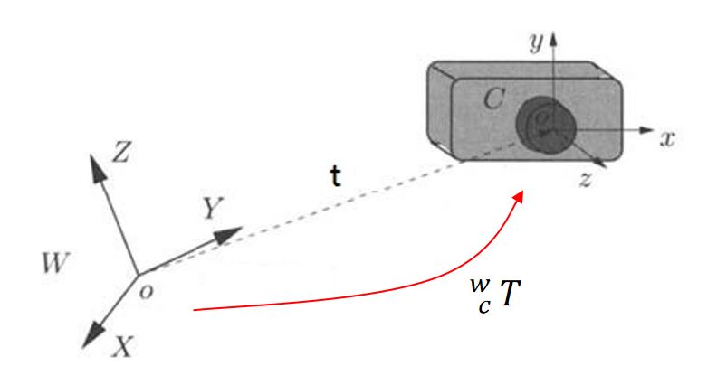
    例如：空间中一点，在相机坐标系中为 $^cP$，求其在世界坐标系中的坐标 $^wP$，则有 $^wP = R \bm{\cdot} {^cP} + t$

    其中，坐标系 {W} -> {C} 就是一个刚体变换，可记为 $^w_cT$

                 

1.2  约束分析 

    $R$ 和 $t$ 共有 12 个未知数，但 R 是标准正交矩阵，自带 6 个约束方程，则刚体变换有 12 - 6 = 6 个自由度 (和直观的感受一致)

    表面上看，似乎只需 2 组空间对应点，联立 6 个方程，便可求得 6 个未知数，但这 6 个方程是有冗余的 (因为这 2 组对应点，在各自的坐标系下，两点之间的距离是相等的)

    因此，第 2 组对应点，只是提供了 2 个约束方程，加上第 1 组对应点的 3 个约束，共有 5 个独立的方程

    显然，还需要第 3 组对应点，提供 1 个独立的方程，才能求出 R 和 t

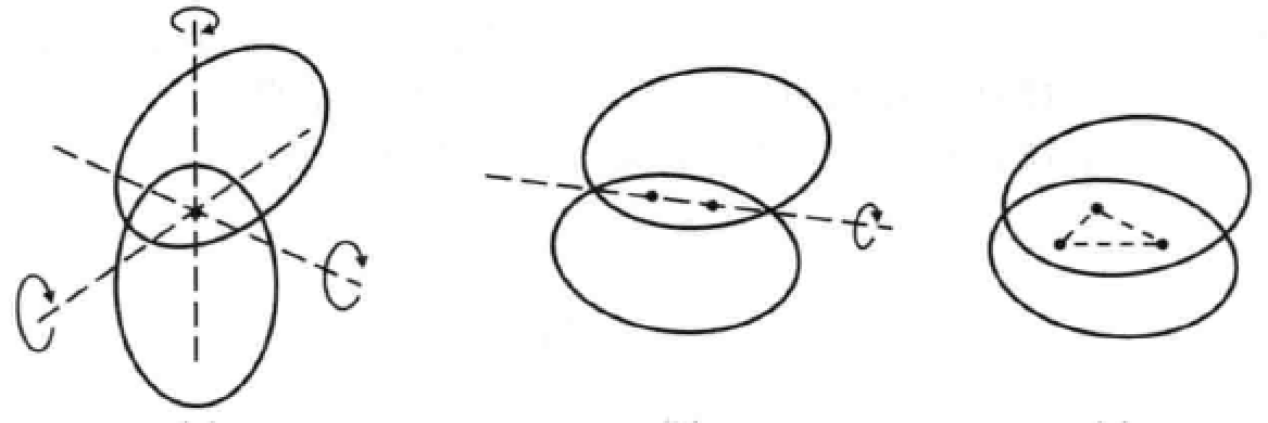
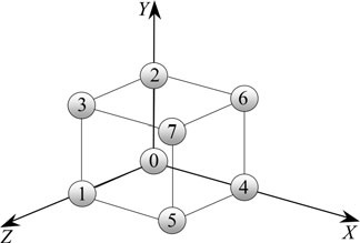
    如图所示，两个刚体之间：1个点重合 => 3个自由度；2个点重合 => 1个自由度；3个点重合=> 0个自由度  

        

    OpenCV 中有一个函数 estimateAffine3D() 可求解刚体变换的矩阵

1.3  直观理解

    一个单位立方体，可在 X-Y-Z 坐标系中自由运动，则运动前后的转换关系，可视为刚体变换

    单点重合：当立方体的角点 0 和 X-Y-Z 坐标系的原点 O 重合时，立方体还能自由的旋转 (X 轴 -> Y 轴 -> Z 轴)

                                           

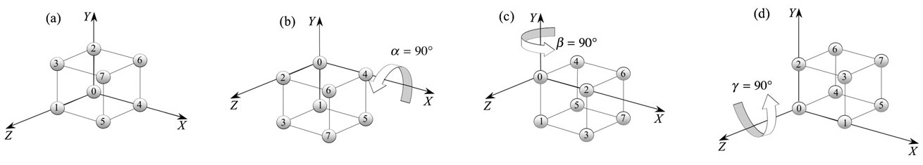
    两点重合：除了立方体的角点 0 和坐标系的 原点 O 重合外，再令角点 4 和 X 轴上的某点重合，则此时立方体只能 绕 X 轴旋转

                    

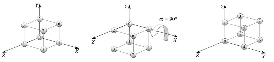
    三点重合：除了以上两个角点 0 和 4，如果再使角点 1 和 Z 轴上的某点重合，则立方体就会和 X-Y-Z 坐标系 牢牢的连接在一起

                       

    因此，选取不共面的三组对应点，联立方程组，便可求得 R 和 T  

   

2  旋转向量

    任意的旋转，都可用一个旋转轴 (axis) 和 绕轴旋转角 (angle) 来描述，简称“轴角”

        

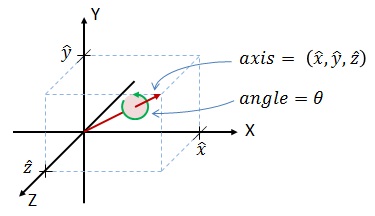
    因此，可用一个方向和旋转轴一致，长度等于旋转角的向量来表示旋转，这个向量称为旋转向量 (或“旋量”)

    假定旋转轴  $\mathbf{n} = [r_{x}, r_{y}, r_{z}]$，旋转角  $\theta$，则旋转向量为 $\theta \mathbf{n}$；旋转向量到旋转矩阵的转换，可由罗德里格斯公式实现，如下：

    $\quad R = cos(\theta) I + (1 - cos \theta) \mathbf{nn^T} + sin \theta \begin{bmatrix} 0&-r_z&r_y \\ r_z&0&-r_x \\ -r_y&r_x&0 \end{bmatrix}$

    反之，从旋转矩阵到旋量，公式如下：

    $\quad \sin \theta \begin{bmatrix}0 &-r_z&r_y \\r_z&0&-r_x \\-r_y & r_x &0 \end{bmatrix} = \dfrac{R - R^T}{2}$

    OpenCV 中有一个 Rodrigues() 函数，可实现二者的相互转换         

?

1 2 3 4 5

void  Rodrigues (       InputArray   src,  // 输入旋转向量 n(3x1 或 1x3) 或 旋转矩阵 R(3x3)       OutputArray  dst,  // 输出旋转矩阵 R 或 旋转向量 n       OutputArray  jacobian = noArray()  // 可选，输出 Jacobian 矩阵(3x9 或 9x3) )

　　　 

3  欧拉角

3.1  定义

    假定平面内有一点 P， 旋转 $\theta$ 角到 $P^{\prime}$ 位置，如下图：    

         

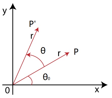
    取 $\angle$POX = $\theta_0$，列方程组得

    $\quad x^{\prime} = r \cos (\theta_0 + \theta) = r \cos \theta_0 \cos\theta - r \sin \theta_0 \sin\theta = x \cos\theta - y \sin \theta$ 

    $\quad y^{\prime} = r \sin(\theta_0+ \theta) = r \sin\theta_0 cos \theta + r \cos \theta_0 \sin\theta = x \sin \theta + y \cos \theta$ 

    转化为矩阵形式  $\begin{bmatrix} x' \\ y' \end{bmatrix} = \begin{bmatrix} cos \theta & -sin \theta \\ sin \theta & cos \theta \end{bmatrix} \begin{bmatrix} x \\ y \end{bmatrix}$

3.2  欧拉角

    将二维旋转矩阵 $R_{2 \times 2}$ 扩展到三维空间

    1）绕 Z 轴旋转 roll，则添加 z 坐标 $\pmb{R_z} = \begin{bmatrix} cos \theta_z & -sin \theta_z & 0 \\ sin \theta_z & cos \theta_z & 0 \\ 0&0&1 \end{bmatrix}$

           

    2）绕 Y 轴旋转 yaw，则添加 y 坐标  $\pmb{R_y} = \begin{bmatrix} cos \theta_y & 0 & \color{blue}{sin \theta_y} \\ 0 & 1 & 0 \\ \color{blue}{-sin \theta_y} & 0 & cos \theta_y \end{bmatrix}$

           

    3）绕 X 轴旋转 pitch，则添加 x 坐标  $\pmb{R_x} = \begin{bmatrix} 1 & 0 & 0 \\ 0 &cos \theta_x & -sin \theta_x \\ 0 & sin \theta_x & cos \theta_x \end{bmatrix}$

           

    因此，当按 Z-Y-X 的顺序旋转时，一个旋转矩阵就被分解成了绕不同轴的三次旋转，旋转角称为 "欧拉角"

    $\quad R = R_z \cdot R_y \cdot R_x = \begin{bmatrix} cos \theta_y cos \theta_z & sin \theta_x sin \theta_y cos \theta_z - cos \theta_x sin \theta_z & sin \theta_x sin \theta_z + cos \theta_x sin \theta_y cos \theta_z \\ cos \theta_y sin \theta_z & cos \theta_x cos \theta_z + sin \theta_x sin \theta_y sin \theta_z & cos \theta_x sin \theta_y sin \theta_z - sin \theta_x cos \theta_z \\ -sin \theta_y & sin \theta_x cos \theta_y & cos \theta_x cos \theta_y \end{bmatrix}$，

    注意：在使用欧拉角时，要先指明旋转的顺序，因为绕不同的轴旋转时得到的欧拉角也不同

    反之，由旋转矩阵求解欧拉角，则有：

    $\quad \theta_x = tan^{-1} (\dfrac{r_{32}}{r_{33}})$

    $\quad \theta_y = sin^{-1} (-r_{33})$

    $\quad \theta_z = tan^{-1} (\dfrac{r_{21}}{r_{11}})$ 

3.3  代码实现

    已知绕三个轴旋转的欧拉角，要转换为旋转矩阵，直接套用公式

?

1 2 3 4 5 6 7 8 9 10 11 12 13 14 15 16 17 18 19 20 21 22 23 24 25

Mat eulerAnglesToRotationMatrix(Vec3f &theta) {     // Calculate rotation about x axis     Mat R_x = (Mat_<double>(3,3) <<                1,       0,              0,                0,       cos(theta[0]),   -sin(theta[0]),                0,       sin(theta[0]),   cos(theta[0])  );       // Calculate rotation about y axis     Mat R_y = (Mat_<double>(3,3) <<                cos(theta[1]),    0,      sin(theta[1]),                0,                1,      0,                -sin(theta[1]),   0,      cos(theta[1])  );       // Calculate rotation about z axis     Mat R_z = (Mat_<double>(3,3) <<                cos(theta[2]),    -sin(theta[2]),      0,                sin(theta[2]),    cos(theta[2]),       0,                0,                0,                   1  );       // Combined rotation matrix     Mat R = R_z * R_y * R_x;       return R; }

    旋转矩阵到欧拉角的转换，要指明旋转顺序 (Z-Y-X 或 X-Y-Z 等 6 种)，下面代码实现了和 MATLAB 中 rotm2euler 一样的功能，只是旋转顺序不同 (X-Y-Z)

?

1 2 3 4 5 6 7 8 9 10 11 12 13 14 15 16 17 18 19 20 21 22 23 24 25 26 27 28 29 30

// Checks if a matrix is a valid rotation matrix. bool isRotationMatrix(Mat &R) {     Mat Rt;     transpose(R, Rt);     Mat shouldBeIdentity = Rt * R;     Mat I = Mat::eye(3,3, shouldBeIdentity.type());       return  norm(I, shouldBeIdentity) < 1e-6; }   // The result is the same as MATLAB except the order of the euler angles ( x and z are swapped ). Vec3f rotationMatrixToEulerAngles(Mat &R) {     assert(isRotationMatrix(R));     float sy = sqrt(R.at<double>(0,0) * R.at<double>(0,0) +  R.at<double>(1,0) * R.at<double>(1,0) );     bool singular = sy < 1e-6; // If       float x, y, z;     if (!singular) {         x = atan2(R.at<double>(2,1) , R.at<double>(2,2));         y = atan2(-R.at<double>(2,0), sy);         z = atan2(R.at<double>(1,0), R.at<double>(0,0));     } else {         x = atan2(-R.at<double>(1,2), R.at<double>(1,1));         y = atan2(-R.at<double>(2,0), sy);         z = 0;     }     return Vec3f(x, y, z); }

 

4  四元数

4.1  定义

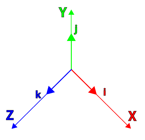
    四元数本质是一种高阶的复数，普通复数有一个实部和一个虚部，而四元数有一个实部和三个虚部

    $\quad q = s + x \mathbf{i} + y \mathbf{j} + z \mathbf{k}$，其中 $\mathbf{i}^2=\mathbf{j}^2=\mathbf{k}^2=\mathbf{ijk}=-1$

        

    平面中任一点的旋转，可通过“左乘” 旋转向量来表示，如下：

    $\quad p = a + b \mathbf{i}$，$q = cos \theta + \mathbf{i} sin \theta$ 

    $\quad p^{\prime} = qp = a\cos\theta-b\sin\theta+(a\sin\theta+b\cos\theta)i$

    推及空间中任一点的旋转，可通过“左乘”四元数来表示，如下：

    $\quad p = [0, a \mathbf{i} + b \mathbf{j} + c \mathbf{k}]$，$q = [cos \theta, sin \theta \mathbf{v}  ]$，其中 $\mathbf{v}$ 由 $\mathbf{i}, \mathbf{j}, \mathbf{k}$ 组合而成

    $\quad p^{\prime} = qp$

4.2  实例

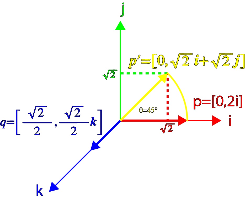
    例1：当向量 p 围绕 k 轴在 i-j 平面内旋转 45°，表示该旋转的四元数为

    $\quad q = \left[\dfrac{\sqrt{2}}{2}, \dfrac{\sqrt{2}}{2} \mathbf{k} \right]$

    取 $p = [0, 2 \mathbf{i}]$，则 $p^{\prime} = qp = [0, \sqrt{2}\mathbf{i} + \sqrt{2} \mathbf{j}]$，如下图 p' 确实是 p 围绕 $\mathbf{k}$ 轴旋转 45° 得到的

         

    例2：当向量 p 围绕 q 旋转 45°，且 q 中的向量 v 在 i-k 平面内和 p 成 45° 时，表示该旋转的四元数为

    $\quad q = \left[ \dfrac{\sqrt{2}}{2},  \dfrac{\sqrt{2}}{2} \left(\dfrac{\sqrt{2}}{2} \mathbf{i} + \dfrac{\sqrt{2}}{2} \mathbf{k} \right) \right]$

    取 $p = [0, 2 \mathbf{i}]$，则 $p^{\prime} = qp = [-1,\sqrt{2}\mathbf{i}+\mathbf{j}]$，可看出 $p^{\prime}$ 中向量模长为 $\sqrt{3}$，这不再是一个纯旋转的变换

        

    但如果再“右乘” $q^{-1}$，则 $p^{\prime} = qpq^{-1} = [0,\mathbf{i}+\sqrt{2}\mathbf{j}+\mathbf{k} ]$，如下图，这又变成了一个纯旋转，但是旋转的角度是 90° 不是 45° 

        

     综上所述，向量 p 围绕任一轴 $\mathbf{v}$ 旋转 $\theta$，则表示该旋转的四元数形式为

     $\quad q=\left[\cos\dfrac{\theta}{2},\sin\dfrac{\theta}{2} \mathbf{v}\right]$    

4.3  转换关系

    假定四元数 $q = s + x \mathbf{i} + y \mathbf{j} + z \mathbf{k}$，则旋转矩阵为

    $\quad R = \begin{bmatrix}1-2(y^{2}+z^{2})&2(xy-sz)&2(xz+sy)\\2(xy+sz)&1-2(x^{2}+z^{2})&2(yz-sx)\\2(xz-sy)&2(yz+sx)&1-2(x^{2}+y^{2})\end{bmatrix}$

    或另一种形式

    $\quad R = \begin{bmatrix} s^2 + x^2 - y^2 -z^2 & 2(xy - sz) & 2(xz + sy) \\ 2(xy +sz) & s^2-x^2+y^2-z^2 & 2(yz - sx) \\ 2(xz-sy) & 2(yz+sx) & s^2-x^2-y^2+z^2 \end{bmatrix}$

    OpenCV 中实现的函数 quat2rot() 如下：   

?

1 2 3 4 5 6 7 8 9 10 11 12 13 14 15 16 17 18 19 20 21 22 23 24 25 26 27

// R = quat2rot(q) // q - 4x1 unit quaternion <qw, qx, qy, qz> // R - 3x3 rotation matrix static Mat quat2rot(const Mat& q) {     CV_Assert(q.type() == CV_64FC1 && q.rows == 4 && q.cols == 1);       double qw = q.at<double>(0,0);     double qx = q.at<double>(1,0);     double qy = q.at<double>(2,0);     double qz = q.at<double>(3,0);       Mat R(3, 3, CV_64FC1);     R.at<double>(0, 0) = 1 - 2*qy*qy - 2*qz*qz;     R.at<double>(0, 1) = 2*qx*qy - 2*qz*qw;     R.at<double>(0, 2) = 2*qx*qz + 2*qy*qw;       R.at<double>(1, 0) = 2*qx*qy + 2*qz*qw;     R.at<double>(1, 1) = 1 - 2*qx*qx - 2*qz*qz;     R.at<double>(1, 2) = 2*qy*qz - 2*qx*qw;       R.at<double>(2, 0) = 2*qx*qz - 2*qy*qw;     R.at<double>(2, 1) = 2*qy*qz + 2*qx*qw;     R.at<double>(2, 2) = 1 - 2*qx*qx - 2*qy*qy;       return R; }

     反之，由旋转矩阵转换为四元数，其实现函数 rot2quat() 如下：

?

1 2 3 4 5 6 7 8 9 10 11 12 13 14 15 16 17 18 19 20 21 22 23 24 25 26 27 28 29 30 31 32 33 34 35 36 37 38 39 40 41

// q = rot2quat(R) // q - 4x1 unit quaternion <qw, qx, qy, qz> // R - 3x3 rotation matrix static Mat rot2quat(const Mat& R) {     CV_Assert(R.type() == CV_64FC1 && R.rows >= 3 && R.cols >= 3);       double m00 = R.at<double>(0,0), m01 = R.at<double>(0,1), m02 = R.at<double>(0,2);     double m10 = R.at<double>(1,0), m11 = R.at<double>(1,1), m12 = R.at<double>(1,2);     double m20 = R.at<double>(2,0), m21 = R.at<double>(2,1), m22 = R.at<double>(2,2);     double trace = m00 + m11 + m22;       double qw, qx, qy, qz;     if (trace > 0) {         double S = sqrt(trace + 1.0) * 2; // S=4*qw         qw = 0.25 * S;         qx = (m21 - m12) / S;         qy = (m02 - m20) / S;         qz = (m10 - m01) / S;     } else if (m00 > m11 && m00 > m22) {         double S = sqrt(1.0 + m00 - m11 - m22) * 2; // S=4*qx         qw = (m21 - m12) / S;         qx = 0.25 * S;         qy = (m01 + m10) / S;         qz = (m02 + m20) / S;     } else if (m11 > m22) {         double S = sqrt(1.0 + m11 - m00 - m22) * 2; // S=4*qy         qw = (m02 - m20) / S;         qx = (m01 + m10) / S;         qy = 0.25 * S;         qz = (m12 + m21) / S;     } else {         double S = sqrt(1.0 + m22 - m00 - m11) * 2; // S=4*qz         qw = (m10 - m01) / S;         qx = (m02 + m20) / S;         qy = (m12 + m21) / S;         qz = 0.25 * S;     }       return (Mat_<double>(4,1) << qw, qx, qy, qz); }

 

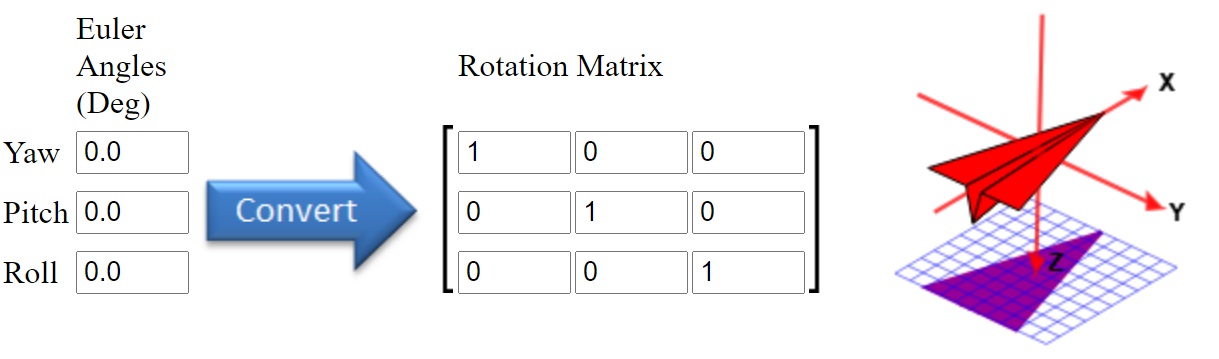
备注1 - 欧拉角可视化

   一个欧拉角的可视化链接 Euler Angle Visualization Tool，输入欧拉角可实时显示位姿变化

          

备注2

    ceres solver 中，提供了一个 rotation.h 的文件，可以方便的实现欧拉角、旋转矩阵和四元数之间的相互转换，链接如下

     ceres solver 中的欧拉角、旋转矩阵和四元数

 

参考

  《An Invitaton to 3D Vision》 ch2

  《Robot Vision》ch13

    OpenCV - 3D rigid/afine transforamtion

    Understanding Quaternions

    Rotation Matrix To Euler Angles

    An Orge compatible class for euler angles