OpenCV 之 图像几何变换

  二维平面中，图像的几何变换有等距、相似、仿射、投影等，如下所示：

    

 

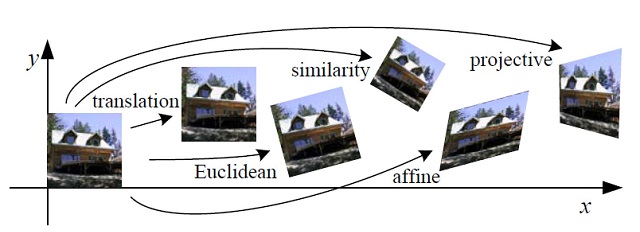
1  图像几何变换

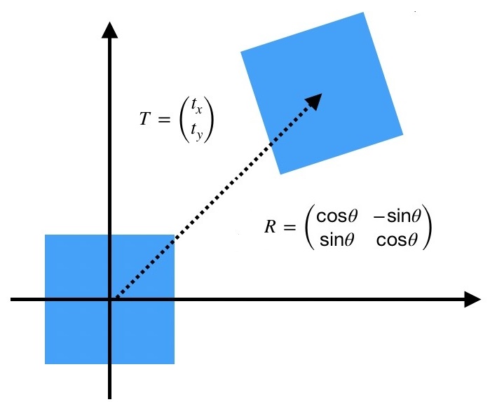
1.1  等距变换

    等距变换 (Isometric Transformation)，是一种二维的刚体变换，可理解为旋转和平移的组合

   $\quad \begin{bmatrix} x^{\prime} \\ y^{\prime} \\ 1 \end{bmatrix} = \begin{bmatrix} \cos \theta & -\sin \theta & t_x \\ \sin \theta & \cos \theta & t_y \\ 0&0&1 \end{bmatrix} \begin{bmatrix} x \\ y \\ 1\end{bmatrix}  =\begin{bmatrix} R_{2 \times 2} & T_{2 \times 1} \\ 0_{1 \times 2} & 1_{1 \times 1} \end{bmatrix} \begin{bmatrix} x \\ y \\1 \end{bmatrix}$

    其中， $R=\begin{bmatrix} \cos \theta &-\sin\theta \\ \sin \theta & \cos \theta \end{bmatrix}$ 为旋转矩阵， $T=\begin{bmatrix}t_x \\ t_y \end{bmatrix}$ 为平移矩阵

    想象一个无限大的平面上，放一张极薄的图片，让它只能在平面内做旋转和平移运动，则这样的运动就是等距变换

    

1.2  相似变换

  相似变换 (Similarity Transformation)，是一个等距变换和各向均匀缩放的组合

   $\quad \begin{bmatrix} x' \\ y' \\ 1 \end{bmatrix} = \begin{bmatrix} s \cos \theta & -s\sin \theta & t_x \\ s \sin \theta & s \cos \theta & t_y \\ 0&0&1 \end{bmatrix} \begin{bmatrix} x \\ y \\ 1\end{bmatrix} = \begin{bmatrix} sR_{2 \times 2} & T_{2 \times 1} \\ 0_{1 \times 2} & 1_{1 \times 1} \end{bmatrix} \begin{bmatrix} x \\ y \\1 \end{bmatrix}$，其中 $s$ 为缩放系数

   想象平面内的一张图片，在旋转和平移的过程中，其大小也会均匀缩放(各个方向)，则这样的变换就是相似变换

     

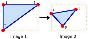
1.3  仿射变换

1.3.1  定义

    仿射变换（Affine Transformation)，是一个非奇异线性变变换 (矩阵乘法) 和 平移变换 (向量加法) 的组合

    矩阵表达式为 $\quad \begin{bmatrix} x' \\ y' \\ 1 \end{bmatrix} = \begin{bmatrix} a_{11} & a_{12} & t_x \\ a_{21} & a_{22} & t_y \\ 0 & 0 & 1 \end{bmatrix} \begin{bmatrix} x \\ y \\ 1 \end{bmatrix} =\begin{bmatrix} A_{2 \times 2} & T_{2 \times 1} \\ 0_{1 \times 2} & 1_{1 \times 1} \end{bmatrix} \begin{bmatrix} x \\ y \\1 \end{bmatrix}$

    其中，当 $A = \begin{bmatrix} a_{11} & a_{12} \\ a_{21} & a_{22} \end{bmatrix}$ 是非奇异时，称 $A$ 为仿射矩阵

1.3.2  分解

    仿射矩阵 $A$ 可分解为：旋转和各向 (正交) 非均匀缩放

    $\quad A = R(\theta) R(-\phi) D R(\phi)$，其中 $D = \begin{bmatrix} \lambda_1 & 0 \\ 0 & \lambda_2 \end{bmatrix}$是一个对角矩阵

    首先，旋转角度 $\phi$；然后在 $x$ 和 $y$ 方向上 (其中 $x\perp y$) 分别缩放 $\lambda_1$ 和 $\lambda_2$；再旋转角度 $-\phi$，也即回转 $\phi$；最后旋转角度 $\theta$

    本质上，平面中的仿射变换，就是奇异值分解的过程：$A=UDV^T$

    

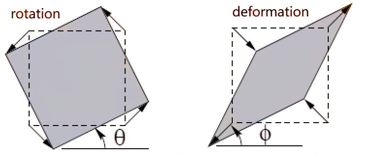
    想象无限大光滑平面内的一张图片，在旋转和平移的过程中，其大小在正交方向上非均匀缩放，则这样的变换就是仿射变换

1.3.3  不变量

    仿射变换的过程中，有三个重要的不变量，分别是：平行线，平行线段长度比，面积比

 

2  OpenCV 函数    

2.1  矩阵 - 相似变换

    对于相似变换，有 4 个未知数 ($s, \theta, t_x, t_y$)，对应 OpenCV 中的 getRotationMatrix2D() 函数    

  Mat getRotationMatrix2D (
      Point2f     center,  // 原图像中的旋转中心点
      double      angle,   // 旋转角度(正值代表逆时针旋转)
      double      scale    // 均匀缩放系数
  )　　

    该函数可得到如下矩阵：

    $\begin{bmatrix} \alpha & \beta & (1- \alpha ) \cdot \texttt{center.x} - \beta \cdot \texttt{center.y} \\ - \beta & \alpha & \beta \cdot \texttt{center.x} + (1- \alpha ) \cdot \texttt{center.y} \end{bmatrix}$

    其中， $\alpha=scale \cdot \cos angle$

                $\beta=scale \cdot \sin angle$

2.2  矩阵 - 仿射变换

    仿射变换有 6 个未知数 ($\phi, \theta, \lambda_1, \lambda_2, t_x, t_y$)，需列 6 组方程，而一组对应特征点 $(x,y)$ -> $(x′,y′)$ 可构造 2 个方程，因此，求解 6 个未知数，需要 3 组对应特征点

        

    OpenCV 中 getAffineTransform() 可求解 2x3 矩阵 $\begin{bmatrix} a_{11} & a_{12} & t_{x} \\ a_{21} & a_{22} & t_y \end{bmatrix}$     

  Mat getAffineTransform (
      const Point2f    src[],  // 原图像的三角顶点坐标
      const Point2f    dst[]   // 目标图像的三角顶点坐标
  )   　　

    其代码实现比较简单，先构建方程组，再利用 solve() 求解 $Ax=b$   

Mat getAffineTransform(const Point2f src[], const Point2f dst[])
{
    Mat M(2, 3, CV_64F), X(6, 1, CV_64F, M.ptr());
    double a[6 * 6], b[6];
    Mat A(6, 6, CV_64F, a), B(6, 1, CV_64F, b);

    for (int i = 0; i < 3; i++)
    {
        int j = i * 12;
        int k = i * 12 + 6;
        a[j] = a[k + 3] = src[i].x;
        a[j + 1] = a[k + 4] = src[i].y;
        a[j + 2] = a[k + 5] = 1;
        a[j + 3] = a[j + 4] = a[j + 5] = 0;
        a[k] = a[k + 1] = a[k + 2] = 0;
        b[i * 2] = dst[i].x;
        b[i * 2 + 1] = dst[i].y;
    }

    solve(A, B, X);
    return M;
}　　

2.3  变换后图象 

     已知仿射变换矩阵 M ，利用 warpAffine() 函数，可得变换后的图像：$\texttt{dst} (x,y) = \texttt{src} ( \texttt{M} _{11} x + \texttt{M} _{12} y + \texttt{M} _{13}, \texttt{M} _{21} x + \texttt{M} _{22} y + \texttt{M} _{23})$ 

void warpAffine(
    InputArray      src,    // 输入图象
    OutputArray     dst,    // 输出图像(大小为 dsize，类型同 src)
    InputArray       M,     // 2x3 矩阵
    Size            dsize,  // 输出图像的大小
    int  flags = INTER_LINEAR,
    int  borderMode = BORDER_CONSTANT,
    const Scalar& borderValue = Scalar()
)　　

    

3  代码示例

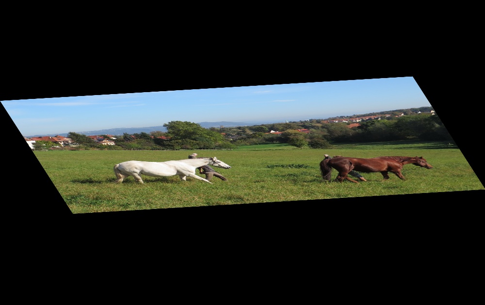
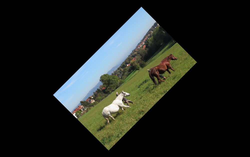
    首先构造3组三角顶点坐标，代入 getAffineTransform() 得到仿射变换的矩阵；再用 getRotationMatrix2D() 构造相似变换的矩阵；

    然后，warpAffine() 求解经过相似变换和仿射变换的图像；最后，显示对比变换后的目标图像

#include "opencv2/imgproc.hpp"
#include "opencv2/imgcodecs.hpp"
#include "opencv2/highgui.hpp"

using namespace cv;

int main()
{
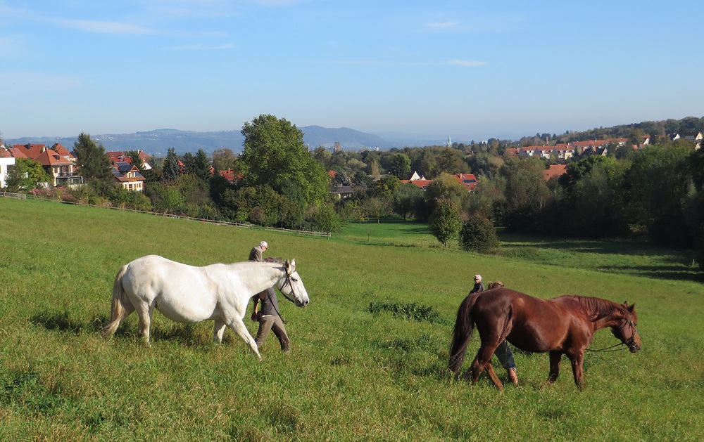
    // 1) read image
    Mat src = imread("horse.jpg");
    
    // 2) triangle vertices
    Point2f srcTri[3];
    srcTri[0] = Point2f(0.f, 0.f);
    srcTri[1] = Point2f(src.cols - 1.f, 0.f);
    srcTri[2] = Point2f(0.f, src.rows - 1.f);

    Point2f dstTri[3];
    dstTri[0] = Point2f(0.f, src.rows * 0.33f);
    dstTri[1] = Point2f(src.cols * 0.85f, src.rows * 0.25f);
    dstTri[2] = Point2f(src.cols * 0.15f, src.rows * 0.7f);

    // 3-1) getAffineTransform
    Mat warp_m1 = getAffineTransform(srcTri, dstTri);

    // 3-2) getRotationMatrix2D
    Mat warp_m2 = getRotationMatrix2D(Point2f(0.5*src.cols, 0.5*src.rows), 45, 0.5);
    
    // 4) warpAffine image
    Mat dst1,dst2;
    warpAffine(src, dst1, warp_m1, Size(src.cols, src.rows));
    warpAffine(src, dst2, warp_m2, Size(src.cols, src.rows));
    
    // 5) show image
    imshow("image", src);
    imshow("warp affine 1", dst1);
    imshow("warp affine 2", dst2);
    waitKey();    
}　　

      结果对比如下：

               

 

参考

    《Computer Vision: Algorithms and Applications》 Chapter 2 Image Formation

    《Multiple View Geometry in Computer Vision》   2.4  A hierarchy of transformations

    OpenCV Tutorials / Image Processing (imgproc module) / Affine Transformations

    OpenCV-Python Tutorials / Image Processing in OpenCV / Geometric Transformations of Images