损失函数

损失函数

• 概述：
  在机器学习和深度学习中，损失函数（Loss Function）用于衡量模型预测值与真实值之间的差异。它是训练过程中优化的目标，通过最小化损失函数来提升模型的性能。
  也叫"代价函数"（Cost Function）或"目标函数"（Objective Function）或"误差函数"（Error Function）。

损失函数名称	PyTorch实现	主要特点
多分类交叉熵损失（Categorical Cross-Entropy Loss）	CrossEntropyLoss()	结合Softmax，适用于多类别分类
二分类交叉熵损失（Binary Cross-Entropy Loss）	BCELoss()	结合Sigmoid，适用于二分类任务
均方误差损失（Mean Squared Error Loss）	MSELoss()	对异常值敏感，梯度连续
平均绝对误差损失（Mean Absolute Error Loss）	L1Loss()	对异常值鲁棒，零点不可导
Smooth L1损失（Smooth L1 Loss）	SmoothL1Loss()	结合L1和L2优点，常用于目标检测

多分类交叉熵损失函数

在多分类任务中，通常使用softmax函数将模型输出的原始分数（logits）转换为概率分布的形式，因此多分类的交叉熵损失也常被称为softmax损失。它的计算方法如下：

对于单个样本：

\[L(\theta) = - \sum_{i=1}^{C} y_i \log(S(f_\theta(x))_i) \]

对于包含 N 个样本的批次：

\[L(\theta) = -\frac{1}{N} \sum_{n=1}^{N} \sum_{i=1}^{C} y_{n,i} \log(S(f_\theta(x_n))_i) \]

其中：

• C：类别总数
• $ y_i $：真实标签的独热编码（第 i 类为 1，其余为 0），表示样本 x 属于某个类别的真实概率
• $ f_\theta(x) $：模型对于输入 x 的原始输出（logits），可以看作加权求和后的结果
• S：Softmax 激活函数
• $ S(f_\theta(x))_i $：模型预测的第 i 类概率

Softmax 函数定义为：

\[S(\mathbf{z})_i = \frac{e^{z_i}}{\sum_{j=1}^{C} e^{z_j}} \]

示例说明：

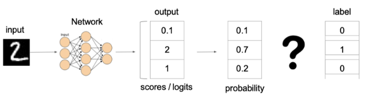
上图中的交叉熵损失为：

\[-(0 \times \log(0.10) + 1 \times \log(0.7) + 0 \times \log(0.2)) = -\log(0.7) \]

从概率角度理解，我们的目标是最小化正确类别所对应的预测概率的对数的负值（使损失值最小），也就是说，损失函数的结果等于正确类别所对应的预测概率的对数的负值的最小化。

实际应用注意：torch.nn.CrossEntropyLoss() 已经将 softmax 激活和交叉熵损失计算合并在一起，因此在使用这个损失函数时，模型的输出层不需要再添加 softmax 激活函数。

# 多分类交叉熵损失函数
criterion = torch.nn.CrossEntropyLoss()  # reduction='mean' 默认值

# 假设有3个样本，类别数为4 -> 即公式中的f(x)
outputs = torch.tensor([[2.0, 1.0, 0.1, 0.5],
                        [0.5, 2.5, 0.3, 0.2],
                        [1.0, 0.2, 0.3, 3.0]])  # 模型的输出（logits），即预测值
# 即公式中的 y
targets = torch.tensor([0, 1, 3])  # 真实标签（类别的索引）
# 注意：也可以使用one-hot编码形式
# targets = torch.tensor([[1, 0, 0, 0],
#                         [0, 1, 0, 0],
#                         [0, 0, 0, 1]])  # 真实标签（one-hot编码形式）

loss = criterion(outputs, targets)  # 参数1: 模型输出（预测值） 参数2: 真实标签
print(f'CrossEntropyLoss: {loss.item()}')

二分类交叉熵损失函数

在处理二分类任务时，我们通常使用 sigmoid 激活函数将模型输出转换为概率值，相应地使用二分类交叉熵损失函数：

\[L = -y \log(\hat{y}) - (1-y) \log(1-\hat{y}) \]

对于包含 N 个样本的批次：

\[L = -\frac{1}{N} \sum_{n=1}^{N} [y_n \log(\hat{y}_n) + (1-y_n) \log(1-\hat{y}_n)] \]

其中：

1. y 是样本 x 属于某个类别的真实概率（0 或 1）
2. \(\hat{y}\) 是模型预测的样本属于某个类别的概率（通过 sigmoid 函数得到）
3. L 用于衡量真实值 y 与预测值 \(\hat{y}\) 之间的差异

Sigmoid 函数定义为：

\[\sigma(z) = \frac{1}{1 + e^{-z}} \]

实际应用注意：torch.nn.BCELoss() 本身不包含 sigmoid 激活函数，因此在将模型输出传递给该损失函数之前，需要先手动应用 sigmoid 函数将输出转换为概率值。或者可以使用 torch.nn.BCEWithLogitsLoss()，它已经将 sigmoid 激活和二分类交叉熵损失合并在一起。

# 二分类交叉熵损失函数
criterion = torch.nn.BCELoss()  # reduction='mean' 默认值
# 假设有3个样本
outputs = torch.tensor([0.9, 0.2, 0.8], dtype=torch.float)  # 模型的输出（已经过sigmoid处理），即预测概率 (0~1之间)
targets = torch.tensor([0, 1, 0], dtype=torch.float)  # 真实标签 (0或1)

loss = criterion(outputs, targets)  # 参数1: 模型输出（预测值） 参数2: 真实标签
print(f'BCELoss: {loss.item()}')

# 或者使用BCEWithLogitsLoss，它包含sigmoid激活
criterion2 = torch.nn.BCEWithLogitsLoss()
outputs_logits = torch.tensor([2.2, -1.4, 1.4], dtype=torch.float)  # 模型的原始输出（logits）
loss2 = criterion2(outputs_logits, targets)
print(f'BCEWithLogitsLoss: {loss2.item()}')

回归任务损失函数

平均绝对误差损失函数（MAE/L1 Loss）

平均绝对误差损失（Mean Absolute Error Loss，MAE），也称为 L1 Loss，以绝对误差作为距离度量。损失函数公式如下：

对于单个样本：

\[L = |y - f_\theta(x)| \]

对于包含 N 个样本的批次：

\[L = \frac{1}{N} \sum_{i=1}^{N} |y_i - f_\theta(x_i)| \]

特点：

1. 由于 L1 损失具有稀疏性，常作为正则项添加到其他损失函数中作为约束，以惩罚较大的值。
2. L1 损失的最大问题是梯度在零点不平滑（不可导），可能导致优化过程跳过极小值点。
3. 相比于 L2 损失，L1 损失对异常值（离群点）更鲁棒。

均方误差损失函数（MSE/L2 Loss）

均方误差损失（Mean Squared Error Loss，MSE），也称为 L2 Loss 或欧氏距离，以误差的平方和的均值作为距离度量。损失函数公式如下：

对于单个样本：

\[L = (y - f_\theta(x))^2 \]

对于包含 N 个样本的批次：

\[L = \frac{1}{N} \sum_{i=1}^{N} (y_i - f_\theta(x_i))^2 \]

特点：

1. L2 损失也常作为正则项使用（如权重衰减）。
2. 当预测值与真实值相差很大时，梯度容易爆炸，对异常值敏感。
3. 相比于 L1 损失，L2 损失在零点处梯度连续且平滑，有利于优化过程。

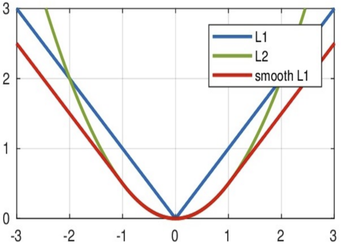
Smooth L1 损失函数

Smooth L1 损失函数 是 L1 损失的光滑版本，它结合了 L1 和 L2 损失的优点。损失函数公式如下：

对于单个样本，定义误差 \(\delta = f_\theta(x) - y\)：

\[\text{SmoothL1}(\delta) = \begin{cases} 0.5 \delta^2 / \beta, & \text{if } |\delta| < \beta \\ |\delta| - 0.5 \beta, & \text{otherwise} \end{cases} \]

对于包含 N 个样本的批次：

\[L = \frac{1}{N} \sum_{i=1}^{N} \text{SmoothL1}(f_\theta(x_i) - y_i) \]

其中 \(\beta\) 是一个超参数，通常取值为 1.0。当 \(\beta = 1\) 时，公式简化为：

\[\text{SmoothL1}(\delta) = \begin{cases} 0.5 \delta^2, & \text{if } |\delta| < 1 \\ |\delta| - 0.5, & \text{otherwise} \end{cases} \]

特点：

1. 在 \([-\beta, \beta]\) 区间内，实际上是 L2 损失，解决了 L1 损失在零点不光滑的问题。
2. 在 \([-\beta, \beta]\) 区间外，实际上是 L1 损失，解决了 L2 损失对离群点梯度爆炸的问题。
3. 这种分段设计使得损失函数在误差较小时具有平滑的梯度，有利于收敛；在误差较大时梯度不会过大，对异常值更鲁棒。

应用场景：常用于目标检测（如 Faster R-CNN、YOLO 等模型中的边界框回归）、人脸关键点检测等回归任务。

# PyTorch 中回归损失函数的使用示例
criterion_l1 = torch.nn.L1Loss()          # 平均绝对误差损失函数
criterion_mse = torch.nn.MSELoss()        # 均方误差损失函数
criterion_smoothl1 = torch.nn.SmoothL1Loss()  # smooth L1损失函数，默认beta=1.0

# 假设有3个样本
outputs = torch.tensor([2.5, 1.8, 3.2], dtype=torch.float)  # 模型的预测值
targets = torch.tensor([2.0, 2.0, 3.0], dtype=torch.float)  # 真实值

loss_l1 = criterion_l1(outputs, targets)
loss_mse = criterion_mse(outputs, targets)
loss_smoothl1 = criterion_smoothl1(outputs, targets)

print(f'L1 Loss: {loss_l1.item()}')
print(f'MSE Loss: {loss_mse.item()}')
print(f'Smooth L1 Loss: {loss_smoothl1.item()}')