1 #导入房价数据
2 from sklearn.datasets import load_boston
3 boston = load_boston()
4 boston.keys()
5 print(boston.DESCR)
6 data = boston.data #查看数据
7 boston.target #查看房价
8 boston.feature_names #特征
1 #一元线性回归模型
2 import pandas
3 pandas.DataFrame(boston.data) #转化为数据框
4 #预处理获取斜率
5 from sklearn.linear_model import LinearRegression
6 LineR = LinearRegression()
7 x = boston.data[:,5]
8 y = boston.target
9 LineR.fit(x.reshape(-1,1),y)
10 w = LineR.coef_ #获取斜率
11 b = LineR.intercept_ #获取截距
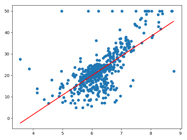
12 #图形化显示
13 import matplotlib.pyplot as plt
14 plt.scatter(x,y)
15 plt.plot(x,w*x+b,'r')
16 plt.show()
![]()
1 #多元线性回归方程
2 # 划分数据集
3 from sklearn.model_selection import train_test_split
4 x_train, x_test, y_train, y_test = train_test_split(boston.data,boston.target,test_size=0.3)
5 # 建立多项式性回归模型
6 LineT = LinearRegression()
7 LineT.fit(x_train,y_train)
8 #检测模型好坏
9 import numpy
10 x_predict = LineT.predict(x_test)
11 #预测的均方误差
12 print("预测的均方误差:",numpy.mean(x_predict - y_test)**2)
13 #模型的分数
14 print("模型的分数:",LineT.score(x_test,y_test))
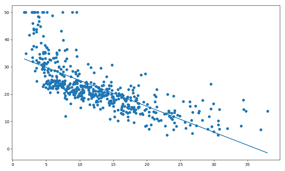
15 #图形化显示
16 x = boston.data[:,12].reshape(-1,1)
17 y = boston.target
18 plt.figure(figsize=(10,6))
19 plt.scatter(x,y)
20 LineT.fit(x,y)
21 y_pred = LineT.predict(x)
22 plt.plot(x,y_pred)
23 print(LineT.coef_,LineT.intercept_)
24 plt.show()
![]()
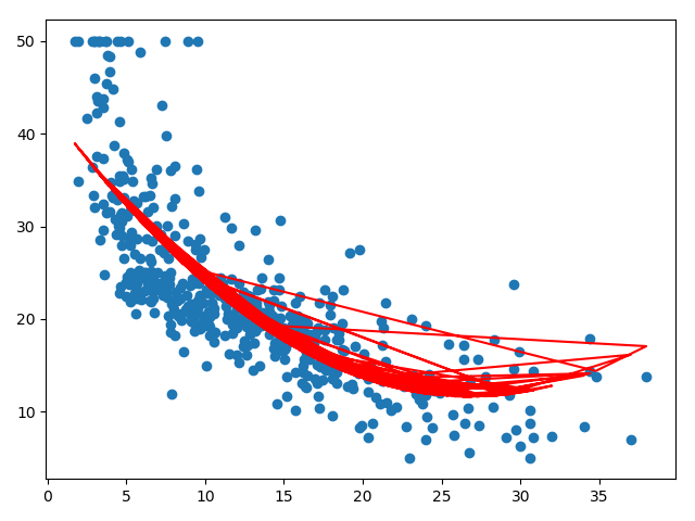
1 #一元多项式回归模型
2 from sklearn.preprocessing import PolynomialFeatures
3 poly = PolynomialFeatures(degree=2)
4 x_poly = poly.fit_transform(x)
5 lr = LinearRegression() #构建模型
6 lr.fit(x_poly, y)
7 y_poly_pred = lr.predict(x_poly)
8 plt.scatter(x, y)
9 plt.plot(x, y_poly_pred, 'r')
10 plt.show()
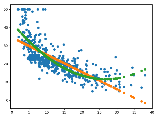
11
12 lrp = LinearRegression()
13 lrp.fit(x_poly, y)
14 plt.scatter(x, y)
15 plt.scatter(x, y_pred)
16 plt.scatter(x, y_poly_pred) # 多项回归
17 plt.show()
![]()
![]()


 浙公网安备 33010602011771号