LOAM笔记及A-LOAM源码阅读
导读
下面是我对LOAM论文的理解以及对A-LOAM的源码阅读(中文注释版的A-LOAM已经push到github,见A-LOAM-NOTED),最后也会手推一下LOAM源码中高斯牛顿法(论文中说的是LM法)求解ICP配准的非线性最小二乘问题,这一部分在A-LOAM代码中用Ceres优化函数库做了简化,CSDN也有篇不错的博文,知乎也有篇很赞的文章,如有问题,欢迎在评论区讨论。
码字绘图不易,转载请注明出处:https://www.cnblogs.com/wellp/p/8877990.html
一、Paper Reading
1. 综述
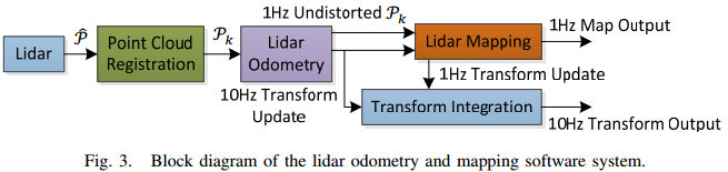
LOAM是一个激光里程计算法,没有闭环检测,也就没有加入图优化框架,该算法把SLAM问题分为两个算法并行运行:一个odometry算法,10Hz;另一个mapping算法,1Hz,最终将两者输出的pose做整合,实现10Hz的位姿实时输出。两个算法都是使用点云中提取出尖锐的边点和平整的面点作为特征点,然后进行特征点匹配,来估计lidar的位姿以及对位姿进行fine tune。匹配特征点时,不是简单的点到点,而是edge point到edge line(点到线)以及planar point到planar patch(点到面),在后续运动估计中建立的残差距离也就是点到线的距离以及点到面的距离,所以感觉LOAM匹配的过程就像是一个点到线以及点到面相结合的ICP算法;需要注意的是odometry和mapping算法的edge line和planar patch(即匹配时的target)的确定略有不同,具体看第3小结的介绍。
2. odometry算法
1)输入是已经消除畸变(所谓的消除畸变,也解释为运动补偿,就是把Pk点云中的所有的点都映射到同一个时刻tk+1,消除由于车辆运动和lidar的旋转导致的点云畸变现象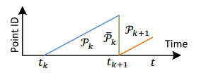 )的上一次扫描的点云
 、此次扫描过程中逐渐被观测到的点云Pk+1、[tk+1, t]时刻的pose之间的增量
  (也解释为pose之间的transform);
2)如果是一次新的扫描就让 等于0;
等于0;
3)然后从点云Pk+1中提取边点和平面点作为特征点,分别构成边特征点集合 和面特征点集合
 ;
;
4)对于集合中的每一个边点以及平面点我们找到在的对应边和对应平面,然后根据(11)式,构建点到线和点到面的距离残差方程,进而估计Lidar的运动,其中优化变量是,优化目标是残差距离,即求一个最优的,使得点到线以及点到面的距离最小;
5)每个残差方程都分配一个权重,特征点到对应边(或者对应面)的距离越大就分配越小的权重,如果距离大于一定阈值,就把权重设置成0;
6)利用LM法(源码中用的是高斯牛顿法)对这个非线性最小二乘问题进行求解,得到,这样就可以更新 ;
7)当非线性优化收敛或者迭代次数到达预设值后,break;
8)如果本次odometry算法已经到达一次扫描的结束时刻就把Pk+1的所有点映射到tk+2时刻得到![]() ,完成对Pk+1点云的运动补偿,否则就只输出已经更新的,为下一次的odometry算法做准备。
,完成对Pk+1点云的运动补偿,否则就只输出已经更新的,为下一次的odometry算法做准备。
论文中的伪代码如下:

3. mapping算法
1)mapping算法就是将已经消除畸变的 点云先转换到全局坐标系变成
 ,然后与局部地图(local map或者称为submap,源码中使用的是三维栅格cube做的局部地图管理)做特征匹配,将配准好的点云添加到
 中,一旦超过预设的范围,就删除范围外的点云,源码中submap的范围是250m * 250m * 150m,需要注意的是,源码中对submap的管理并不是基于时序的滑动窗口方式,而是空间范围划分方式,这就是为什么最后的frame对应的submap会包含早期的frames:
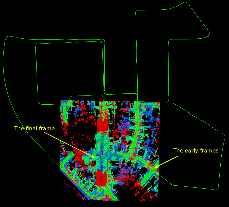
这种submap方式比基于时序的滑动窗口方式会包含更多的历史帧信息,对于点云配准更友好,当然这也就导致内存占用增加;
2)mapping算法中,从中提取特征点的方式跟之前一样,也就是根据曲率值判断一个点是边点还是面点,但是特征点的数量是odometry算法的10倍,具体通过调整曲率值的比较阈值实现,源码中其实也不是10倍了,反正就是比odometry算法提取的特征点会多;
3)然后就是匹配,即在Qk中找特征点的correspondence,在odometry算法中,correspondence的确定是为了最快的计算速度,使用的是基于最近邻的思路来找对应线以及对应面,具体为:最近邻的2个边点构成对应边edge line、最近邻的3个面点构成对应面planar patch;而mapping算法是通过对特征点周围的点云簇(源码是使用了最近邻的5个点作为点云簇)进行PCA主成分分析(求点云簇的协方差矩阵的特征值和特征向量),来确定找到对应边edge line的方向向量以及确定对应面planar patch的法向量。correspondence确定后的优化求解过程就跟之前一样了,实现将配准到局部地图,进而达到对odometry算法计算出的位姿进行fine tune的目的。
4. 系统整体过程
这里主要说下mapping输出的1Hz位姿和odometry输出的10Hz位姿的整合过程:当mapping计算出一个位姿Pmap后,就跟与之时间同步的一个odometry位姿Podom计算增量△P = Pmap * Podom-1,然后用△P去修正后续的高频odometry位姿,修正后的10Hz高频位姿就是LOAM最终输出的实时位姿,然后直到mapping算法再计算出一个位姿后重复上述过程。
二、A-LOAM源码阅读
1. 节点图
先放一个运行A-LOAM时的ros节点图,整体架构如代码一般清晰。
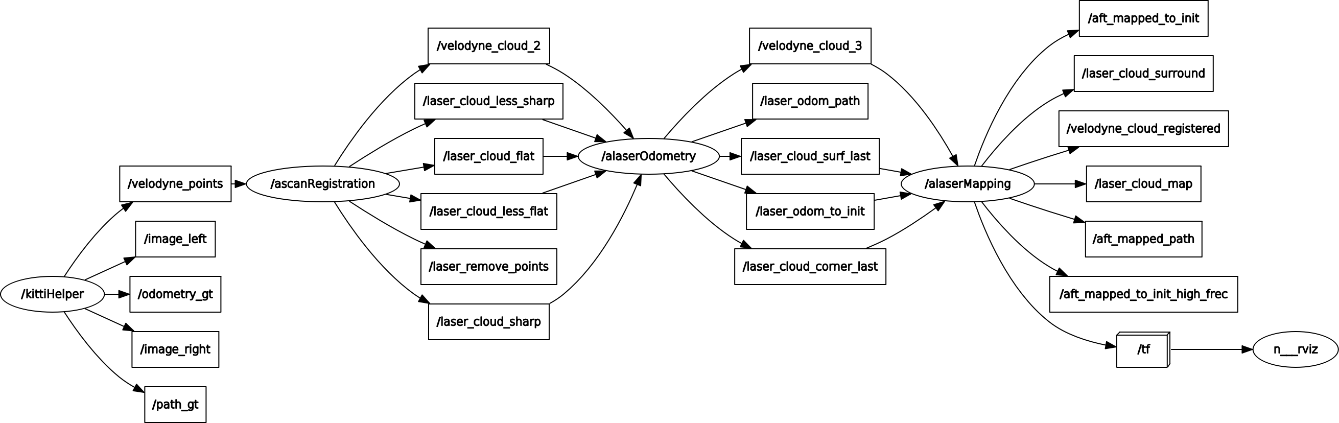
2. 代码整体综述
A-LOAM的代码清晰度确实很高,整理的非常简洁,主要是使用了Ceres函数库代替了张继手推的ICP优化求解部分(用Ceres的自动求导,代替了手推的解析求导,效率会低一些)。整个代码目录如下:
 |
docker目录 | 提供了docker环境,方便开发者搭建环境 |
| include目录 | 包含一个简单的通用头文件以及一个计时器的类TicToc,计时单位为ms | |
| launch目录 | ros的启动文件 | |
| out、picture目录 | 预留的编译产出目录、README.md中的图片 | |
| rviz_cfg目录 | rviz的配置文件 | |
| src目录 | 核心代码:4个cpp分别对应了1.节点图中的4个node;1个hpp为基于Ceres构建残差函数时使用的各个仿函数类(是不是命名成Functor,更直观?) |
3.kittiHelper.cpp
1)对应节点:/kittiHelper
2)功能:读取kitti odometry的数据集的数据,具体包括点云、左右相机的图像、以及pose的groundtruth(训练集才有),然后分成5个topic以10Hz(可修改)的频率发布出去,其中真正对算法有用的topic只有点云/velodyne_points,其他四个topic都是在rviz中可视化用。
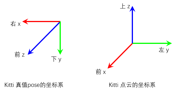
3)代码分析:这部分代码主要是ros的消息发布,需要注意的是,kitti的训练集真值pose的坐标系和点云的坐标系不相同如下图所示,A-LOAM为了统一,坐标系均采用点云的坐标系,所以需要将真值pose进行坐标变换,转到点云的坐标系下;真值pose的坐标系实际是左相机的坐标系。
A-LOAM在此处还存在一个坐标变换的bug,如下所示,当然这个bug只会影响可视化真值轨迹时的姿态,并不影响后续算法的运行,其实更准确的应该使用KITTI提供的左相机与Lidar的标定参数进行变换;
Eigen::Quaterniond q_w_i(gt_pose.topLeftCorner<3, 3>());
// Eigen::Quaterniond q = q_transform * q_w_i;// 此处应该添加 * q_transform.inverse(),如下所示,其实更准确的应该使用KITTI提供的左相机到Lidar的标定参数进行变换
Eigen::Quaterniond q = q_transform * q_w_i *q_transform.inverse();
q.normalize();
Eigen::Vector3d t = q_transform * gt_pose.topRightCorner<3, 1>();
4.scanRegistration.cpp
1)对应节点:/ascanRegistration
2)功能:对输入点云进行滤波,提取4种feature,即边缘点特征sharp、less_sharp,面特征flat、less_flat
3)代码分析:
main函数主要是订阅前一个节点发布的点云topic,一旦接受到一帧点云就执行一次回调函数laserCloudHandler,所以重点来看该回调函数
// 首先对点云滤波,去除NaN值的无效点,以及在Lidar坐标系原点MINIMUM_RANGE距离以内的点
pcl::removeNaNFromPointCloud(laserCloudIn, laserCloudIn, indices);
removeClosedPointCloud(laserCloudIn, laserCloudIn, MINIMUM_RANGE);
(假设64线Lidar的水平角度分辨率是0.2deg,则每个scan理论有360/0.2=1800个点,为方便叙述,我们称每个scan点的ID为fireID,即fireID [0~1799],相应的scanID [0~63] )
接下来通过Lidar坐标系下点的仰角以及水平夹角计算点云的scanID和fireID,需要注意的是这里的计算方式其实并不适用kitti数据集的点云,因为kitti的点云已经被运动补偿过。
point.intensity = scanID + scanPeriod * relTime;// intensity字段的整数部分存放scanID,小数部分存放归一化后的fireID
laserCloudScans[scanID].push_back(point); // 将点根据scanID放到对应的子点云laserCloudScans中
然后将子点云laserCloudScans合并成一帧点云laserCloud,注意这里的单帧点云laserCloud可以认为已经是有序点云了,按照scanID和fireID的顺序存放
for (int i = 0; i < N_SCANS; i++)
{
    scanStartInd[i] = laserCloud->size() + 5;// 记录每个scan的开始index,忽略前5个点
    *laserCloud += laserCloudScans[i];
    scanEndInd[i] = laserCloud->size() - 6;// 记录每个scan的结束index,忽略后5个点,开始和结束处的点云容易产生不闭合的“接缝”,对提取edge feature不利
}
接下来计算点的曲率
for (int i = 5; i < cloudSize - 5; i++)
{
     float diffX = laserCloud->points[i - 5].x + laserCloud->points[i - 4].x + laserCloud->points[i - 3].x + laserCloud->points[i - 2].x + laserCloud->points[i - 1].x - 10 * laserCloud->points[i].x + laserCloud->points[i + 1].x + laserCloud->points[i + 2].x + laserCloud->points[i + 3].x + laserCloud->points[i + 4].x + laserCloud->points[i + 5].x;
     float diffY = laserCloud->points[i - 5].y + laserCloud->points[i - 4].y + laserCloud->points[i - 3].y + laserCloud->points[i - 2].y + laserCloud->points[i - 1].y - 10 * laserCloud->points[i].y + laserCloud->points[i + 1].y + laserCloud->points[i + 2].y + laserCloud->points[i + 3].y + laserCloud->points[i + 4].y + laserCloud->points[i + 5].y;
     float diffZ = laserCloud->points[i - 5].z + laserCloud->points[i - 4].z + laserCloud->points[i - 3].z + laserCloud->points[i - 2].z + laserCloud->points[i - 1].z - 10 * laserCloud->points[i].z + laserCloud->points[i + 1].z + laserCloud->points[i + 2].z + laserCloud->points[i + 3].z + laserCloud->points[i + 4].z + laserCloud->points[i + 5].z;

     cloudCurvature[i] = diffX * diffX + diffY * diffY + diffZ * diffZ;
     cloudSortInd[i] = i;
     cloudNeighborPicked[i] = 0;// 点有没有被选选择为feature点
     cloudLabel[i] = 0;// Label 2: corner_sharp
                       // Label 1: corner_less_sharp, 包含Label 2
                       // Label -1: surf_flat
                       // Label 0: surf_less_flat, 包含Label -1,因为点太多,最后会降采样
}
下面的一个大的for loop就是根据曲率计算4种特征点
for (int i = 0; i < N_SCANS; i++)// 按照scan的顺序提取4种特征点
{
    if (scanEndInd[i] - scanStartInd[i] < 6)// 如果该scan的点数少于7个点,就跳过
        continue;
    pcl::PointCloud<PointType>::Ptr surfPointsLessFlatScan(new pcl::PointCloud<PointType>);
    for (int j = 0; j < 6; j++)// 将该scan分成6小段执行特征检测
    {
        int sp = scanStartInd[i] + (scanEndInd[i] - scanStartInd[i]) * j / 6;// subscan的起始index
        int ep = scanStartInd[i] + (scanEndInd[i] - scanStartInd[i]) * (j + 1) / 6 - 1;// subscan的结束index

        TicToc t_tmp;
        std::sort(cloudSortInd + sp, cloudSortInd + ep + 1, comp);// 根据曲率有小到大对subscan的点进行sort
        t_q_sort += t_tmp.toc();

        int largestPickedNum = 0;
        for (int k = ep; k >= sp; k--)// 从后往前,即从曲率大的点开始提取corner feature
        {
            int ind = cloudSortInd[k];

            if (cloudNeighborPicked[ind] == 0 &&
                cloudCurvature[ind] > 0.1)// 如果该点没有被选择过,并且曲率大于0.1
            {
                largestPickedNum++;
                if (largestPickedNum <= 2)// 该subscan中曲率最大的前2个点认为是corner_sharp特征点
                {
                    cloudLabel[ind] = 2;
                    cornerPointsSharp.push_back(laserCloud->points[ind]);
                    cornerPointsLessSharp.push_back(laserCloud->points[ind]);
                }
                else if (largestPickedNum <= 20)// 该subscan中曲率最大的前20个点认为是corner_less_sharp特征点
                {
                    cloudLabel[ind] = 1;
                    cornerPointsLessSharp.push_back(laserCloud->points[ind]);
                }
                else
                {
                    break;
                }

                cloudNeighborPicked[ind] = 1;// 标记该点被选择过了

                // 与当前点距离的平方 <= 0.05的点标记为选择过,避免特征点密集分布
                for (int l = 1; l <= 5; l++)
                {
                    float diffX = laserCloud->points[ind + l].x - laserCloud->points[ind + l - 1].x;
                    float diffY = laserCloud->points[ind + l].y - laserCloud->points[ind + l - 1].y;
                    float diffZ = laserCloud->points[ind + l].z - laserCloud->points[ind + l - 1].z;
                    if (diffX * diffX + diffY * diffY + diffZ * diffZ > 0.05)
                    {
                        break;
                    }

                    cloudNeighborPicked[ind + l] = 1;
                }
                for (int l = -1; l >= -5; l--)
                {
                    float diffX = laserCloud->points[ind + l].x - laserCloud->points[ind + l + 1].x;
                    float diffY = laserCloud->points[ind + l].y - laserCloud->points[ind + l + 1].y;
                    float diffZ = laserCloud->points[ind + l].z - laserCloud->points[ind + l + 1].z;
                    if (diffX * diffX + diffY * diffY + diffZ * diffZ > 0.05)
                    {
                        break;
                    }

                    cloudNeighborPicked[ind + l] = 1;
                }
            }
        }

        // 提取surf平面feature,与上述类似,选取该subscan曲率最小的前4个点为surf_flat
        int smallestPickedNum = 0;
        for (int k = sp; k <= ep; k++)
        {
            int ind = cloudSortInd[k];

            if (cloudNeighborPicked[ind] == 0 &&
                cloudCurvature[ind] < 0.1)
            {

                cloudLabel[ind] = -1;
                surfPointsFlat.push_back(laserCloud->points[ind]);

                smallestPickedNum++;
                if (smallestPickedNum >= 4)
                {
                    break;
                }

                cloudNeighborPicked[ind] = 1;
                for (int l = 1; l <= 5; l++)
                {
                    float diffX = laserCloud->points[ind + l].x - laserCloud->points[ind + l - 1].x;
                    float diffY = laserCloud->points[ind + l].y - laserCloud->points[ind + l - 1].y;
                    float diffZ = laserCloud->points[ind + l].z - laserCloud->points[ind + l - 1].z;
                    if (diffX * diffX + diffY * diffY + diffZ * diffZ > 0.05)
                    {
                        break;
                    }

                    cloudNeighborPicked[ind + l] = 1;
                }
                for (int l = -1; l >= -5; l--)
                {
                    float diffX = laserCloud->points[ind + l].x - laserCloud->points[ind + l + 1].x;
                    float diffY = laserCloud->points[ind + l].y - laserCloud->points[ind + l + 1].y;
                    float diffZ = laserCloud->points[ind + l].z - laserCloud->points[ind + l + 1].z;
                    if (diffX * diffX + diffY * diffY + diffZ * diffZ > 0.05)
                    {
                        break;
                    }

                    cloudNeighborPicked[ind + l] = 1;
                }
            }
        }

        // 其他的非corner特征点与surf_flat特征点一起组成surf_less_flat特征点
        for (int k = sp; k <= ep; k++)
        {
            if (cloudLabel[k] <= 0)
            {
                surfPointsLessFlatScan->push_back(laserCloud->points[k]);
            }
        }
    }

    // 最后对该scan点云中提取的所有surf_less_flat特征点进行降采样,因为点太多了
    pcl::PointCloud<PointType> surfPointsLessFlatScanDS;
    pcl::VoxelGrid<PointType> downSizeFilter;
    downSizeFilter.setInputCloud(surfPointsLessFlatScan);
    downSizeFilter.setLeafSize(0.2, 0.2, 0.2);
    downSizeFilter.filter(surfPointsLessFlatScanDS);

    surfPointsLessFlat += surfPointsLessFlatScanDS;
}
最后就是将当前帧点云提取出的4种特征点与滤波后的当前帧点云进行publish
5.laserOdometry.cpp
1)对应节点:/alaserOdometry
2)功能:基于前述的4种feature进行帧与帧的点云特征配准,即简单的Lidar Odometry
3)代码分析:
a. 先明确几个关键变量的含义
// Lidar Odometry线程估计的frame在world坐标系的位姿P,Transformation from current frame to world frame
Eigen::Quaterniond q_w_curr(1, 0, 0, 0);
Eigen::Vector3d t_w_curr(0, 0, 0);

// 点云特征匹配时的优化变量
double para_q[4] = {0, 0, 0, 1};
double para_t[3] = {0, 0, 0};

// 下面的2个分别是优化变量para_q和para_t的映射:表示的是两个world坐标系下的位姿P之间的增量,例如△P = P0.inverse() * P1
Eigen::Map<Eigen::Quaterniond> q_last_curr(para_q);
Eigen::Map<Eigen::Vector3d> t_last_curr(para_t);
b. 再介绍一下main函数之前的几个函数
TransformToStart:将当前帧Lidar坐标系下的点云变换到上一帧Lidar坐标系下(也就是当前帧的初始位姿,起始位姿,所以函数名是TransformToStart),因为kitti点云已经去除了畸变,所以不再考虑运动补偿。(如果点云没有去除畸变,用slerp差值的方式计算出每个点在fire时刻的位姿,然后进行TransformToStart的坐标变换,一方面实现了变换到上一帧Lidar坐标系下;另一方面也可以理解成点都将fire时刻统一到了开始时刻,即去除了畸变,完成了运动补偿)
之后的5个Handler函数为接受上游5个topic的回调函数,作用是将消息缓存到对应的queue中,以便后续处理。
c. 然后就是main函数,即Odometry线程的核心代码部分:
if (!systemInited)// 第一帧不进行匹配,仅仅将 cornerPointsLessSharp 保存至 laserCloudCornerLast
                  //                   将 surfPointsLessFlat    保存至 laserCloudSurfLast,以及更新对应的kdtree
                  // 为下次匹配提供target
{
    systemInited = true;
    std::cout << "Initialization finished \n";
}
之后一个关键的大for loop:
for (size_t opti_counter = 0; opti_counter < 2; ++opti_counter)// 点到线以及点到面的ICP,迭代2次
{
    ...
}
接着介绍这个for loop里面的内容,关于Ceres的使用,就不介绍了,可以参考Ceres函数库的说明文档,或者高翔的《视觉SLAM十四讲》中的Ceres示例,注意一下优化变量是两个world坐标系下的位姿P的增量para_q和para_t
for (size_t opti_counter = 0; opti_counter < 2; ++opti_counter)// 点到线以及点到面的ICP,迭代2次
{
    corner_correspondence = 0;
    plane_correspondence = 0;

    //ceres::LossFunction *loss_function = NULL;
    ceres::LossFunction* loss_function = new ceres::HuberLoss(0.1);
    ceres::LocalParameterization* q_parameterization =
        new ceres::EigenQuaternionParameterization();
    ceres::Problem::Options problem_options;

    ceres::Problem problem(problem_options);
    problem.AddParameterBlock(para_q, 4, q_parameterization);
    problem.AddParameterBlock(para_t, 3);

    pcl::PointXYZI pointSel;
    std::vector<int> pointSearchInd;
    std::vector<float> pointSearchSqDis;

    TicToc t_data;
    // 基于最近邻(只找2个最近邻点)原理建立corner特征点之间关联,find correspondence for corner features
    for (int i = 0; i < cornerPointsSharpNum; ++i)
    {
        TransformToStart(&(cornerPointsSharp->points[i]), &pointSel);// 将当前帧的corner_sharp特征点O_cur,从当前帧的Lidar坐标系下变换到上一帧的Lidar坐标系下(记为点O,注意与前面的点O_cur不同),以利于寻找corner特征点的correspondence
        kdtreeCornerLast->nearestKSearch(pointSel, 1, pointSearchInd, pointSearchSqDis);// kdtree中的点云是上一帧的corner_less_sharp,所以这是在上一帧
                                                                                        // 的corner_less_sharp中寻找当前帧corner_sharp特征点O的最近邻点(记为A)

        int closestPointInd = -1, minPointInd2 = -1;
        if (pointSearchSqDis[0] < DISTANCE_SQ_THRESHOLD)// 如果最近邻的corner特征点之间距离平方小于阈值,则最近邻点A有效
        {
            closestPointInd = pointSearchInd[0];
            int closestPointScanID = int(laserCloudCornerLast->points[closestPointInd].intensity);

            double minPointSqDis2 = DISTANCE_SQ_THRESHOLD;
            // 寻找点O的另外一个最近邻的点(记为点B) in the direction of increasing scan line
            for (int j = closestPointInd + 1; j < (int)laserCloudCornerLast->points.size(); ++j)// laserCloudCornerLast 来自上一帧的corner_less_sharp特征点,由于提取特征时是
            {                                                                                   // 按照scan的顺序提取的,所以laserCloudCornerLast中的点也是按照scanID递增的顺序存放的
                // if in the same scan line, continue
                if (int(laserCloudCornerLast->points[j].intensity) <= closestPointScanID)// intensity整数部分存放的是scanID
                    continue;

                // if not in nearby scans, end the loop
                if (int(laserCloudCornerLast->points[j].intensity) > (closestPointScanID + NEARBY_SCAN))
                    break;

                double pointSqDis = (laserCloudCornerLast->points[j].x - pointSel.x) *
                    (laserCloudCornerLast->points[j].x - pointSel.x) +
                    (laserCloudCornerLast->points[j].y - pointSel.y) *
                    (laserCloudCornerLast->points[j].y - pointSel.y) +
                    (laserCloudCornerLast->points[j].z - pointSel.z) *
                    (laserCloudCornerLast->points[j].z - pointSel.z);

                if (pointSqDis < minPointSqDis2)// 第二个最近邻点有效,更新点B
                {
                    // find nearer point
                    minPointSqDis2 = pointSqDis;
                    minPointInd2 = j;
                }
            }

            // 寻找点O的另外一个最近邻的点B in the direction of decreasing scan line
            for (int j = closestPointInd - 1; j >= 0; --j)
            {
                // if in the same scan line, continue
                if (int(laserCloudCornerLast->points[j].intensity) >= closestPointScanID)
                    continue;

                // if not in nearby scans, end the loop
                if (int(laserCloudCornerLast->points[j].intensity) < (closestPointScanID - NEARBY_SCAN))
                    break;

                double pointSqDis = (laserCloudCornerLast->points[j].x - pointSel.x) *
                    (laserCloudCornerLast->points[j].x - pointSel.x) +
                    (laserCloudCornerLast->points[j].y - pointSel.y) *
                    (laserCloudCornerLast->points[j].y - pointSel.y) +
                    (laserCloudCornerLast->points[j].z - pointSel.z) *
                    (laserCloudCornerLast->points[j].z - pointSel.z);

                if (pointSqDis < minPointSqDis2)// 第二个最近邻点有效,更新点B
                {
                    // find nearer point
                    minPointSqDis2 = pointSqDis;
                    minPointInd2 = j;
                }
            }
        }
        if (minPointInd2 >= 0) // both closestPointInd and minPointInd2 is valid
        {                      // 即特征点O的两个最近邻点A和B都有效
            Eigen::Vector3d curr_point(cornerPointsSharp->points[i].x,
                cornerPointsSharp->points[i].y,
                cornerPointsSharp->points[i].z);
            Eigen::Vector3d last_point_a(laserCloudCornerLast->points[closestPointInd].x,
                laserCloudCornerLast->points[closestPointInd].y,
                laserCloudCornerLast->points[closestPointInd].z);
            Eigen::Vector3d last_point_b(laserCloudCornerLast->points[minPointInd2].x,
                laserCloudCornerLast->points[minPointInd2].y,
                laserCloudCornerLast->points[minPointInd2].z);

            double s;// 运动补偿系数,kitti数据集的点云已经被补偿过,所以s = 1.0
            if (DISTORTION)
                s = (cornerPointsSharp->points[i].intensity - int(cornerPointsSharp->points[i].intensity)) / SCAN_PERIOD;
            else
                s = 1.0;
            // 用点O,A,B构造点到线的距离的残差项,注意这三个点都是在上一帧的Lidar坐标系下,即,残差 = 点O到直线AB的距离
            // 具体到介绍lidarFactor.cpp时再说明该残差的具体计算方法
            ceres::CostFunction* cost_function = LidarEdgeFactor::Create(curr_point, last_point_a, last_point_b, s);
            problem.AddResidualBlock(cost_function, loss_function, para_q, para_t);
            corner_correspondence++;
        }
    }
    // 下面说的点符号与上述相同
    // 与上面的建立corner特征点之间的关联类似,寻找平面特征点O的最近邻点ABC(只找3个最近邻点),即基于最近邻原理建立surf特征点之间的关联,find correspondence for plane features
    for (int i = 0; i < surfPointsFlatNum; ++i)
    {
        TransformToStart(&(surfPointsFlat->points[i]), &pointSel);
        kdtreeSurfLast->nearestKSearch(pointSel, 1, pointSearchInd, pointSearchSqDis);

        int closestPointInd = -1, minPointInd2 = -1, minPointInd3 = -1;
        if (pointSearchSqDis[0] < DISTANCE_SQ_THRESHOLD)// 找到的最近邻点A有效
        {
            closestPointInd = pointSearchInd[0];

            // get closest point's scan ID
            int closestPointScanID = int(laserCloudSurfLast->points[closestPointInd].intensity);
            double minPointSqDis2 = DISTANCE_SQ_THRESHOLD, minPointSqDis3 = DISTANCE_SQ_THRESHOLD;

            // search in the direction of increasing scan line
            for (int j = closestPointInd + 1; j < (int)laserCloudSurfLast->points.size(); ++j)
            {
                // if not in nearby scans, end the loop
                if (int(laserCloudSurfLast->points[j].intensity) > (closestPointScanID + NEARBY_SCAN))
                    break;

                double pointSqDis = (laserCloudSurfLast->points[j].x - pointSel.x) *
                    (laserCloudSurfLast->points[j].x - pointSel.x) +
                    (laserCloudSurfLast->points[j].y - pointSel.y) *
                    (laserCloudSurfLast->points[j].y - pointSel.y) +
                    (laserCloudSurfLast->points[j].z - pointSel.z) *
                    (laserCloudSurfLast->points[j].z - pointSel.z);

                // if in the same or lower scan line
                if (int(laserCloudSurfLast->points[j].intensity) <= closestPointScanID && pointSqDis < minPointSqDis2)
                {
                    minPointSqDis2 = pointSqDis;// 找到的第2个最近邻点有效,更新点B,注意如果scanID准确的话,一般点A和点B的scanID相同
                    minPointInd2 = j;
                }
                // if in the higher scan line
                else if (int(laserCloudSurfLast->points[j].intensity) > closestPointScanID && pointSqDis < minPointSqDis3)
                {
                    minPointSqDis3 = pointSqDis;// 找到的第3个最近邻点有效,更新点C,注意如果scanID准确的话,一般点A和点B的scanID相同,且与点C的scanID不同,与LOAM的paper叙述一致
                    minPointInd3 = j;
                }
            }

            // search in the direction of decreasing scan line
            for (int j = closestPointInd - 1; j >= 0; --j)
            {
                // if not in nearby scans, end the loop
                if (int(laserCloudSurfLast->points[j].intensity) < (closestPointScanID - NEARBY_SCAN))
                    break;

                double pointSqDis = (laserCloudSurfLast->points[j].x - pointSel.x) *
                    (laserCloudSurfLast->points[j].x - pointSel.x) +
                    (laserCloudSurfLast->points[j].y - pointSel.y) *
                    (laserCloudSurfLast->points[j].y - pointSel.y) +
                    (laserCloudSurfLast->points[j].z - pointSel.z) *
                    (laserCloudSurfLast->points[j].z - pointSel.z);

                // if in the same or higher scan line
                if (int(laserCloudSurfLast->points[j].intensity) >= closestPointScanID && pointSqDis < minPointSqDis2)
                {
                    minPointSqDis2 = pointSqDis;
                    minPointInd2 = j;
                }
                else if (int(laserCloudSurfLast->points[j].intensity) < closestPointScanID && pointSqDis < minPointSqDis3)
                {
                    // find nearer point
                    minPointSqDis3 = pointSqDis;
                    minPointInd3 = j;
                }
            }

            if (minPointInd2 >= 0 && minPointInd3 >= 0)// 如果三个最近邻点都有效
            {

                Eigen::Vector3d curr_point(surfPointsFlat->points[i].x,
                    surfPointsFlat->points[i].y,
                    surfPointsFlat->points[i].z);
                Eigen::Vector3d last_point_a(laserCloudSurfLast->points[closestPointInd].x,
                    laserCloudSurfLast->points[closestPointInd].y,
                    laserCloudSurfLast->points[closestPointInd].z);
                Eigen::Vector3d last_point_b(laserCloudSurfLast->points[minPointInd2].x,
                    laserCloudSurfLast->points[minPointInd2].y,
                    laserCloudSurfLast->points[minPointInd2].z);
                Eigen::Vector3d last_point_c(laserCloudSurfLast->points[minPointInd3].x,
                    laserCloudSurfLast->points[minPointInd3].y,
                    laserCloudSurfLast->points[minPointInd3].z);

                double s;
                if (DISTORTION)
                    s = (surfPointsFlat->points[i].intensity - int(surfPointsFlat->points[i].intensity)) / SCAN_PERIOD;
                else
                    s = 1.0;
                // 用点O,A,B,C构造点到面的距离的残差项,注意这三个点都是在上一帧的Lidar坐标系下,即,残差 = 点O到平面ABC的距离
                // 同样的,具体到介绍lidarFactor.cpp时再说明该残差的具体计算方法
                ceres::CostFunction* cost_function = LidarPlaneFactor::Create(curr_point, last_point_a, last_point_b, last_point_c, s);
                problem.AddResidualBlock(cost_function, loss_function, para_q, para_t);
                plane_correspondence++;
            }
        }
    }

    printf("data association time %f ms \n", t_data.toc());

    if ((corner_correspondence + plane_correspondence) < 10)
    {
        printf("less correspondence! *************************************************\n");
    }

    TicToc t_solver;
    ceres::Solver::Options options;
    options.linear_solver_type = ceres::DENSE_QR;
    options.max_num_iterations = 4;
    options.minimizer_progress_to_stdout = false;
    ceres::Solver::Summary summary;
    // 基于构建的所有残差项,求解最优的当前帧位姿与上一帧位姿的位姿增量:para_q和para_t
    ceres::Solve(options, &problem, &summary);
    printf("solver time %f ms \n", t_solver.toc());
}
printf("optimization twice time %f \n", t_opt.toc());
经过2次点到线以及点到面的ICP点云配准之后,得到最优的位姿增量para_q和para_t,即,q_last_curr和t_last_curr
// 用最新计算出的位姿增量,更新上一帧的位姿,得到当前帧的位姿,注意这里说的位姿都指的是世界坐标系下的位姿
t_w_curr = t_w_curr + q_w_curr * t_last_curr;
q_w_curr = q_w_curr * q_last_curr;
最后就是:
(1)publish由当前Odometry线程计算出的当前帧在世界坐标系在的位姿、corner_less_sharp特征点、surf_less_flat特征点、滤波后的点云(原封不动的转发上一个node处理出(简单滤波)的当前帧点云)
(2) 用cornerPointsLessSharp和surfPointsLessFlat 更新 laserCloudCornerLast和laserCloudSurfLast以及相应的kdtree,为下一次点云特征匹配提供target
最后的最后,说明一下各个节点的计算频率问题:
(1)第1个节点/kittiHelper发布topic的频率设置为10Hz(当然是可以修改的),
(2)下游节点即第2个节点/ascanRegistration,没有设置频率,接收到上游的消息后,进行特征提取,提取完毕后立即publish相关topic,因为特征提取时间一般小于100ms,所以可以认为该节点publish的频率也是10Hz
(3)下下游节点即第3个节点/alaserOdometry,大循环设置的ros::Rate rate(100); 即 100Hz执行一次Odometry(可以理解成100Hz刷一次Odometry,不一定执行,要看buffer中有没有数据,有数据就真正执行1次Odometry),并且为各个接受到的各个topic设置了作为缓存容器的queue,旨在防止执行一次Odometry的时间超过100ms,所以该节点publish的频率允许<=10Hz;需要注意的是在publish特征点和点云时有一个publish频率的设置,这是为了控制最后一个节点的执行频率。
if (frameCount % skipFrameNum == 0)
{
    ...
}
(4)最后一个节点即第4个节点/alaserMapping,没有设置频率,直接ros::spin();了,也就是接受到一次上游节点发布的topic就执行一次回调函数。需要注意的是,该节点的处理时间很有可能会超过100ms,为了实现LOAM算法整体的实时性,该节点虽然也设置了接受topic的缓存容器,但是会清空没有来得及处理的历史缓存消息,详见下一节的介绍。
6.laserMapping.cpp
1)对应节点:/alaserMapping
2)功能:基于前述的corner_less_sharp特征点和surf_less_flat特征点,进行帧与submap的点云特征配准,对Odometry线程计算的位姿进行finetune
3)代码分析:
a. 同样地,先明确几个关键变量的含义
// 点云特征匹配时的优化变量
double parameters[7] = {0, 0, 0, 1, 0, 0, 0};

// Mapping线程估计的frame在world坐标系的位姿P,因为Mapping的算法耗时很有可能会超过100ms,所以
// 这个位姿P不是实时的,LOAM最终输出的实时位姿P_realtime,需要Mapping线程计算的相对低频位姿和
// Odometry线程计算的相对高频位姿做整合,详见后面laserOdometryHandler函数分析。此外需要注意
// 的是,不同于Odometry线程,这里的位姿P,即q_w_curr和t_w_curr,本身就是匹配时的优化变量。
Eigen::Map<Eigen::Quaterniond> q_w_curr(parameters);
Eigen::Map<Eigen::Vector3d> t_w_curr(parameters + 4);

// 下面的两个变量是world坐标系下的Odometry计算的位姿和Mapping计算的位姿之间的增量(也即变换,transformation)
// wmap_odom * wodom_curr = wmap_curr(即前面的q/t_w_curr)
// transformation between odom's world and map's world frame
Eigen::Quaterniond q_wmap_wodom(1, 0, 0, 0);
Eigen::Vector3d t_wmap_wodom(0, 0, 0);

// Odometry线程计算的frame在world坐标系的位姿
Eigen::Quaterniond q_wodom_curr(1, 0, 0, 0);
Eigen::Vector3d t_wodom_curr(0, 0, 0);
b. 再介绍一下main函数之前的几个函数
// set initial guess,上一帧的增量wmap_wodom * 本帧Odometry位姿wodom_curr,旨在为本帧Mapping位姿w_curr设置一个初始值
void transformAssociateToMap()
{
    q_w_curr = q_wmap_wodom * q_wodom_curr;
    t_w_curr = q_wmap_wodom * t_wodom_curr + t_wmap_wodom;
}

// 用在最后,当Mapping的位姿w_curr计算完毕后,更新增量wmap_wodom,旨在为下一次执行transformAssociateToMap函数时做准备
void transformUpdate()
{
    q_wmap_wodom = q_w_curr * q_wodom_curr.inverse();
    t_wmap_wodom = t_w_curr - q_wmap_wodom * t_wodom_curr;
}

// 用Mapping的位姿w_curr,将Lidar坐标系下的点变换到world坐标系下
void pointAssociateToMap(PointType const *const pi, PointType *const po)
{
    Eigen::Vector3d point_curr(pi->x, pi->y, pi->z);
    Eigen::Vector3d point_w = q_w_curr * point_curr + t_w_curr;
    po->x = point_w.x();
    po->y = point_w.y();
    po->z = point_w.z();
    po->intensity = pi->intensity;
    //po->intensity = 1.0;
}

// 这个没有用到,是上面pointAssociateToMap的逆变换,即用Mapping的位姿w_curr,将world坐标系下的点变换到Lidar坐标系下
void pointAssociateTobeMapped(PointType const *const pi, PointType *const po)
{
    Eigen::Vector3d point_w(pi->x, pi->y, pi->z);
    Eigen::Vector3d point_curr = q_w_curr.inverse() * (point_w - t_w_curr);
    po->x = point_curr.x();
    po->y = point_curr.y();
    po->z = point_curr.z();
    po->intensity = pi->intensity;
}
之后的几个Handler函数为接受到上游publish的topic后的回调函数,同样会将消息缓存到对应的queue中,以便后续处理,需要注意的是
// receive odomtry
void laserOdometryHandler(const nav_msgs::Odometry::ConstPtr &laserOdometry)
{
    mBuf.lock();
    odometryBuf.push(laserOdometry);
    mBuf.unlock();

    // high frequence publish
    Eigen::Quaterniond q_wodom_curr;
    Eigen::Vector3d t_wodom_curr;
    q_wodom_curr.x() = laserOdometry->pose.pose.orientation.x;
    ...
    t_wodom_curr.z() = laserOdometry->pose.pose.position.z;

    // 为了保证LOAM整体的实时性,防止Mapping线程耗时>100ms导致丢帧,用上一次的增量wmap_wodom来更新
    // Odometry的位姿,旨在用Mapping位姿的初始值(也可以理解为预测值)来实时输出,进而实现LOAM整体的实时性
    Eigen::Quaterniond q_w_curr = q_wmap_wodom * q_wodom_curr;
    Eigen::Vector3d t_w_curr = q_wmap_wodom * t_wodom_curr + t_wmap_wodom;
    ...
    pubOdomAftMappedHighFrec.publish(odomAftMapped);
}
c. 然后就是核心函数process以及main函数:
main函数比较简单,接收上游节点的topic,定义对应的消息回调函数,然后就进入核心函数process()了,进行Mapping,即帧与submap的匹配,对Odometry计算的位姿进行finetune
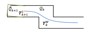
process函数中,我个人觉得最不方便理解的是submap的定义和维护,所以在代码分析之前,先介绍一下LOAM中这个submap,直接上图
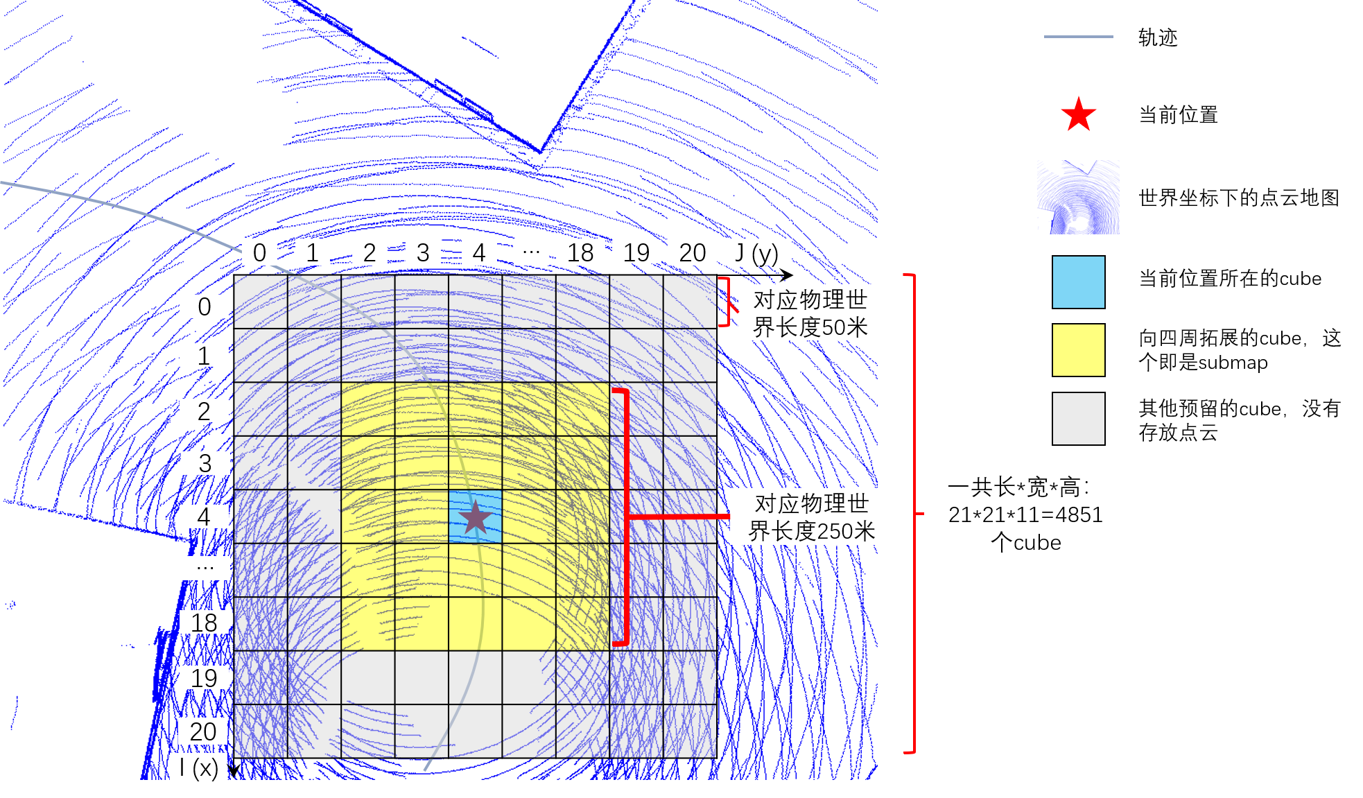
LOAM中Mapping线程中的帧与submap的特征匹配,用到的submap就是上图中的黄色区域,submap中的corner特征和surf特征在匹配中作为target;而当前帧的单帧点云中的两种特征在匹配中作为source。
下面说明一下几个与维护submap有关的全局变量的含义,需要注意的是LOAM对submap中cube的管理都是以1维数组的形式
// cube的总数量,也就是上图中的所有小格子个总数量 21 * 21 * 11 = 4851
const int laserCloudNum = laserCloudWidth * laserCloudHeight * laserCloudDepth;

// 下面两个变量是一模一样的,有点冗余,记录submap中的有效cube的index,注意submap中cube的最大数量为 5 * 5 * 5 = 125
int laserCloudValidInd[125];
int laserCloudSurroundInd[125];

// 存放cube点云特征的数组,数组大小4851,points in every cube
pcl::PointCloud<PointType>::Ptr laserCloudCornerArray[laserCloudNum];
pcl::PointCloud<PointType>::Ptr laserCloudSurfArray[laserCloudNum];
为了保证LOAM算法整体的实时性,Mapping线程每次只处理cornerLastBuf.front()及其他与之时间同步的消息,而因为Mapping线程耗时>100ms导致的历史缓存都会被清空,具体操作如下:
while (!cornerLastBuf.empty() && !surfLastBuf.empty() &&
    !fullResBuf.empty() && !odometryBuf.empty())
{
    mBuf.lock();
    // odometryBuf只保留一个与cornerLastBuf.front()时间同步的最新消息
    while (!odometryBuf.empty() && odometryBuf.front()->header.stamp.toSec() < cornerLastBuf.front()->header.stamp.toSec())
        odometryBuf.pop();
    if (odometryBuf.empty())
    {
        mBuf.unlock();
        break;
    }

    // surfLastBuf也如此
    while (!surfLastBuf.empty() && surfLastBuf.front()->header.stamp.toSec() < cornerLastBuf.front()->header.stamp.toSec())
        surfLastBuf.pop();
    if (surfLastBuf.empty())
    {
        mBuf.unlock();
        break;
    }

    // fullResBuf也如此
    while (!fullResBuf.empty() && fullResBuf.front()->header.stamp.toSec() < cornerLastBuf.front()->header.stamp.toSec())
        fullResBuf.pop();
    if (fullResBuf.empty())
    {
        mBuf.unlock();
        break;
    }

    ...

    // 清空cornerLastBuf的历史缓存,为了LOAM的整体实时性
    while (!cornerLastBuf.empty())
    {
        cornerLastBuf.pop();
        printf("drop lidar frame in mapping for real time performance \n");
    }

    mBuf.unlock();
}
然后是关于submap位置的维护,直接看下面的注释吧:
// 上一帧的增量wmap_wodom * 本帧Odometry位姿wodom_curr,旨在为本帧Mapping位姿w_curr设置一个初始值
transformAssociateToMap();

TicToc t_shift;
// 下面这是计算当前帧位置t_w_curr(在上图中用红色五角星表示的位置)IJK坐标(见上图中的坐标轴),
// 参照LOAM_NOTED的注释,下面有关25呀,50啥的运算,等效于以50m为单位进行缩放,因为LOAM用1维数组
// 进行cube的管理,而数组的index只用是正数,所以要保证IJK坐标都是正数,所以加了laserCloudCenWidth/Heigh/Depth
// 的偏移,来使得当前位置尽量位于submap的中心处,也就是使得上图中的五角星位置尽量处于所有格子的中心附近,
// 偏移laserCloudCenWidth/Heigh/Depth会动态调整,来保证当前位置尽量位于submap的中心处。
int centerCubeI = int((t_w_curr.x() + 25.0) / 50.0) + laserCloudCenWidth;
int centerCubeJ = int((t_w_curr.y() + 25.0) / 50.0) + laserCloudCenHeight;
int centerCubeK = int((t_w_curr.z() + 25.0) / 50.0) + laserCloudCenDepth;

// 由于计算机求余是向零取整,为了不使(-50.0,50.0)求余后都向零偏移,当被求余数为负数时求余结果统一向左偏移一个单位,也即减一
if (t_w_curr.x() + 25.0 < 0)
    centerCubeI--;
if (t_w_curr.y() + 25.0 < 0)
    centerCubeJ--;
if (t_w_curr.z() + 25.0 < 0)
    centerCubeK--;

// 以下注释部分参照LOAM_NOTED,结合我画的submap的示意图说明下面的6个while loop的作用:要
// 注意世界坐标系下的点云地图是固定的,但是IJK坐标系我们是可以移动的,所以这6个while loop
// 的作用就是调整IJK坐标系(也就是调整所有cube位置),使得五角星在IJK坐标系的坐标范围处于
// 3 < centerCubeI < 18, 3 < centerCubeJ < 8, 3 < centerCubeK < 18,目的是为了防止后续向
// 四周拓展cube(图中的黄色cube就是拓展的cube)时,index(即IJK坐标)成为负数。
while (centerCubeI < 3)
{
    for (int j = 0; j < laserCloudHeight; j++)
    {
        for (int k = 0; k < laserCloudDepth; k++)
        {
            int i = laserCloudWidth - 1;
            pcl::PointCloud<PointType>::Ptr laserCloudCubeCornerPointer =
                laserCloudCornerArray[i + laserCloudWidth * j + laserCloudWidth * laserCloudHeight * k];
            pcl::PointCloud<PointType>::Ptr laserCloudCubeSurfPointer =
                laserCloudSurfArray[i + laserCloudWidth * j + laserCloudWidth * laserCloudHeight * k];
            for (; i >= 1; i--)// 在I方向cube[I]=cube[I-1],清空最后一个空出来的cube,实现IJK坐标系向I轴负方向移动一个cube的
                               // 效果,从相对运动的角度看是图中的五角星在IJK坐标系下向I轴正方向移动了一个cube,如下面动图所示,所
                               // 以centerCubeI最后++,laserCloudCenWidth也++,为下一帧Mapping时计算五角星的IJK坐标做准备
            {
                laserCloudCornerArray[i + laserCloudWidth * j + laserCloudWidth * laserCloudHeight * k] =
                    laserCloudCornerArray[i - 1 + laserCloudWidth * j + laserCloudWidth * laserCloudHeight * k];
                laserCloudSurfArray[i + laserCloudWidth * j + laserCloudWidth * laserCloudHeight * k] =
                    laserCloudSurfArray[i - 1 + laserCloudWidth * j + laserCloudWidth * laserCloudHeight * k];
            }
            laserCloudCornerArray[i + laserCloudWidth * j + laserCloudWidth * laserCloudHeight * k] =
                laserCloudCubeCornerPointer;
            laserCloudSurfArray[i + laserCloudWidth * j + laserCloudWidth * laserCloudHeight * k] =
                laserCloudCubeSurfPointer;
            laserCloudCubeCornerPointer->clear();
            laserCloudCubeSurfPointer->clear();
        }
    }

    centerCubeI++;
    laserCloudCenWidth++;
}

while (centerCubeI >= laserCloudWidth - 3)
{
    ...
}

while (centerCubeJ < 3)
{
    ...
}

while (centerCubeJ >= laserCloudHeight - 3)
{
    ...
}

while (centerCubeK < 3)
{
    ...
}

while (centerCubeK >= laserCloudDepth - 3)
{
    ...
}
I轴方向调整一次示意图
生成submap的特征点云如下,需要注意的是,LOAM这种方式生成的submap并不是基于时序的滑动窗口方式,而是基于空间范围划分的方式:
// 下面的两个定义可以认为是清空submap
int laserCloudValidNum = 0;
int laserCloudSurroundNum = 0;
// 向IJ坐标轴的正负方向各拓展2个cube,K坐标轴的正负方向各拓展1个cube,上图中五角星所在的蓝色cube就是当前位置
// 所处的cube,拓展的cube就是黄色的cube,这些cube就是submap的范围
for (int i = centerCubeI - 2; i <= centerCubeI + 2; i++)
{
    for (int j = centerCubeJ - 2; j <= centerCubeJ + 2; j++)
    {
        for (int k = centerCubeK - 1; k <= centerCubeK + 1; k++)
        {
            if (i >= 0 && i < laserCloudWidth &&
                j >= 0 && j < laserCloudHeight &&
                k >= 0 && k < laserCloudDepth)// 如果坐标合法
            {
                // 记录submap中的所有cube的index,记为有效index
                laserCloudValidInd[laserCloudValidNum] = i + laserCloudWidth * j + laserCloudWidth * laserCloudHeight * k;
                laserCloudValidNum++;
                laserCloudSurroundInd[laserCloudSurroundNum] = i + laserCloudWidth * j + laserCloudWidth * laserCloudHeight * k;
                laserCloudSurroundNum++;
            }
        }
    }
}

laserCloudCornerFromMap->clear();
laserCloudSurfFromMap->clear();
for (int i = 0; i < laserCloudValidNum; i++)
{
    // 将有效index的cube中的点云叠加到一起组成submap的特征点云
    *laserCloudCornerFromMap += *laserCloudCornerArray[laserCloudValidInd[i]];
    *laserCloudSurfFromMap += *laserCloudSurfArray[laserCloudValidInd[i]];
}
接下来就是以降采样后的submap特征点云为target,以当前帧降采样后的特征点云为source的ICP过程了,同样地也分为点到线和点到面的匹配,基本流程与Odometry线程相同,不同的是建立correspondence(关联)的方式不同,具体看下面的介绍,先是点到线的ICP过程:
for (int i = 0; i < laserCloudCornerStackNum; i++)
{
    pointOri = laserCloudCornerStack->points[i];
    // 需要注意的是submap中的点云都是world坐标系,而当前帧的点云都是Lidar坐标系,所以
    // 在搜寻最近邻点时,先用预测的Mapping位姿w_curr,将Lidar坐标系下的特征点变换到world坐标系下
    pointAssociateToMap(&pointOri, &pointSel);
    // 在submap的corner特征点(target)中,寻找距离当前帧corner特征点(source)最近的5个点
    kdtreeCornerFromMap->nearestKSearch(pointSel, 5, pointSearchInd, pointSearchSqDis);

    if (pointSearchSqDis[4] < 1.0)
    {
        std::vector<Eigen::Vector3d> nearCorners;
        Eigen::Vector3d center(0, 0, 0);
        for (int j = 0; j < 5; j++)
        {
            Eigen::Vector3d tmp(laserCloudCornerFromMap->points[pointSearchInd[j]].x,
                laserCloudCornerFromMap->points[pointSearchInd[j]].y,
                laserCloudCornerFromMap->points[pointSearchInd[j]].z);
            center = center + tmp;
            nearCorners.push_back(tmp);
        }
        // 计算这个5个最近邻点的中心
        center = center / 5.0;

        // 协方差矩阵
        Eigen::Matrix3d covMat = Eigen::Matrix3d::Zero();
        for (int j = 0; j < 5; j++)
        {
            Eigen::Matrix<double, 3, 1> tmpZeroMean = nearCorners[j] - center;
            covMat = covMat + tmpZeroMean * tmpZeroMean.transpose();
        }

        // 计算协方差矩阵的特征值和特征向量,用于判断这5个点是不是呈线状分布,此为PCA的原理
        Eigen::SelfAdjointEigenSolver<Eigen::Matrix3d> saes(covMat);

        // if is indeed line feature
        // note Eigen library sort eigenvalues in increasing order
        Eigen::Vector3d unit_direction = saes.eigenvectors().col(2);// 如果5个点呈线状分布,最大的特征值对应的特征向量就是该线的方向向量
        Eigen::Vector3d curr_point(pointOri.x, pointOri.y, pointOri.z);
        if (saes.eigenvalues()[2] > 3 * saes.eigenvalues()[1])// 如果最大的特征值 >> 其他特征值,则5个点确实呈线状分布,否则认为直线“不够直”
        {
            Eigen::Vector3d point_on_line = center;
            Eigen::Vector3d point_a, point_b;
            // 从中心点沿着方向向量向两端移动0.1m,构造线上的两个点
            point_a = 0.1 * unit_direction + point_on_line;
            point_b = -0.1 * unit_direction + point_on_line;

            // 然后残差函数的形式就跟Odometry一样了,残差距离即点到线的距离,到介绍lidarFactor.cpp时再说明具体计算方法
            ceres::CostFunction* cost_function = LidarEdgeFactor::Create(curr_point, point_a, point_b, 1.0);
            problem.AddResidualBlock(cost_function, loss_function, parameters, parameters + 4);
            corner_num++;
        }
    }
}
上面的点到线的ICP过程就比Odometry中的要鲁棒和准确一些了(当然也就更耗时一些),因为不是简单粗暴地搜最近的2个corner点作为target的线,而是PCA计算出最近邻的5个点的主方向作为线的方向,而且还会check直线是不是“足够直”,
接着看点到面的ICP过程:
for (int i = 0; i < laserCloudSurfStackNum; i++)
{
    pointOri = laserCloudSurfStack->points[i];

    pointAssociateToMap(&pointOri, &pointSel);

    //也找5个最近邻点
    kdtreeSurfFromMap->nearestKSearch(pointSel, 5, pointSearchInd, pointSearchSqDis);

    // 求面的法向量就不是用的PCA了(虽然论文中说还是PCA),使用的是最小二乘拟合,是为了提效?不确定
    // 假设平面不通过原点,则平面的一般方程为Ax + By + Cz + 1 = 0,用这个假设可以少算一个参数,提效。
    Eigen::Matrix<double, 5, 3> matA0;
    Eigen::Matrix<double, 5, 1> matB0 = -1 * Eigen::Matrix<double, 5, 1>::Ones();
    // 用上面的2个矩阵表示平面方程就是 matA0 * norm(A, B, C) = matB0,这是个超定方程组,因为数据个数超过未知数的个数
    if (pointSearchSqDis[4] < 1.0)
    {
        for (int j = 0; j < 5; j++)
        {
            matA0(j, 0) = laserCloudSurfFromMap->points[pointSearchInd[j]].x;
            matA0(j, 1) = laserCloudSurfFromMap->points[pointSearchInd[j]].y;
            matA0(j, 2) = laserCloudSurfFromMap->points[pointSearchInd[j]].z;
        }
        // 求解这个最小二乘问题,可得平面的法向量,find the norm of plane
        Eigen::Vector3d norm = matA0.colPivHouseholderQr().solve(matB0);
        // Ax + By + Cz + 1 = 0,全部除以法向量的模长,方程依旧成立,而且使得法向量归一化了
        double negative_OA_dot_norm = 1 / norm.norm();
        norm.normalize();

        // Here n(pa, pb, pc) is unit norm of plane
        bool planeValid = true;
        for (int j = 0; j < 5; j++)
        {
            // 点(x0, y0, z0)到平面Ax + By + Cz + D = 0 的距离公式 = fabs(Ax0 + By0 + Cz0 + D) / sqrt(A^2 + B^2 + C^2)
            if (fabs(norm(0) * laserCloudSurfFromMap->points[pointSearchInd[j]].x +
                norm(1) * laserCloudSurfFromMap->points[pointSearchInd[j]].y +
                norm(2) * laserCloudSurfFromMap->points[pointSearchInd[j]].z + negative_OA_dot_norm) > 0.2)
            {
                planeValid = false;// 平面没有拟合好,平面“不够平”
                break;
            }
        }
        Eigen::Vector3d curr_point(pointOri.x, pointOri.y, pointOri.z);
        if (planeValid)
        {
            // 构造点到面的距离残差项,同样的,具体到介绍lidarFactor.cpp时再说明该残差的具体计算方法
            ceres::CostFunction* cost_function = LidarPlaneNormFactor::Create(curr_point, norm, negative_OA_dot_norm);
            problem.AddResidualBlock(cost_function, loss_function, parameters, parameters + 4);
            surf_num++;
        }
    }
}
上面的点到面的ICP过程同样比Odometry中的要鲁棒和准确一些了(当然也就更耗时一些),因为不是简单粗暴地搜最近的3个surf点作为target的平面点,而是对最近邻的5个点进行基于最小二乘的平面拟合,而且还会check拟合出的平面是不是“足够平”,再然后就是匹配之后的一些操作,主要包括更新位姿增量、更新submap:
// 完成ICP(迭代2次)的特征匹配后,用最后匹配计算出的优化变量w_curr,更新增量wmap_wodom,为下一次Mapping做准备
transformUpdate();

TicToc t_add;
// 下面两个for loop的作用就是将当前帧的特征点云,逐点进行操作:转换到world坐标系并添加到对应位置的cube中
for (int i = 0; i < laserCloudCornerStackNum; i++)
{
    // Lidar坐标系转到world坐标系
    pointAssociateToMap(&laserCloudCornerStack->points[i], &pointSel);

    // 计算本次的特征点的IJK坐标,进而确定添加到哪个cube中
    int cubeI = int((pointSel.x + 25.0) / 50.0) + laserCloudCenWidth;
    int cubeJ = int((pointSel.y + 25.0) / 50.0) + laserCloudCenHeight;
    int cubeK = int((pointSel.z + 25.0) / 50.0) + laserCloudCenDepth;

    if (pointSel.x + 25.0 < 0)
        cubeI--;
    if (pointSel.y + 25.0 < 0)
        cubeJ--;
    if (pointSel.z + 25.0 < 0)
        cubeK--;

    if (cubeI >= 0 && cubeI < laserCloudWidth &&
        cubeJ >= 0 && cubeJ < laserCloudHeight &&
        cubeK >= 0 && cubeK < laserCloudDepth)
    {
        int cubeInd = cubeI + laserCloudWidth * cubeJ + laserCloudWidth * laserCloudHeight * cubeK;
        laserCloudCornerArray[cubeInd]->push_back(pointSel);
    }
}

for (int i = 0; i < laserCloudSurfStackNum; i++)
{
    ...
}
printf("add points time %f ms\n", t_add.toc());

TicToc t_filter;
// 因为新增加了点云,对之前已经存有点云的cube全部重新进行一次降采样
// 这个地方可以简单优化一下:如果之前的cube没有新添加点就不需要再降采样
for (int i = 0; i < laserCloudValidNum; i++)
{
    int ind = laserCloudValidInd[i];

    pcl::PointCloud<PointType>::Ptr tmpCorner(new pcl::PointCloud<PointType>());
    downSizeFilterCorner.setInputCloud(laserCloudCornerArray[ind]);
    downSizeFilterCorner.filter(*tmpCorner);
    laserCloudCornerArray[ind] = tmpCorner;

    pcl::PointCloud<PointType>::Ptr tmpSurf(new pcl::PointCloud<PointType>());
    downSizeFilterSurf.setInputCloud(laserCloudSurfArray[ind]);
    downSizeFilterSurf.filter(*tmpSurf);
    laserCloudSurfArray[ind] = tmpSurf;
}
printf("filter time %f ms \n", t_filter.toc());
最后就是publish一些topic,可以在rviz中接受可视化点云、轨迹的结果。需要注意的最后求出的位姿不是KITTI真值位姿的坐标系,如果需要利用真值位姿进行评测还得进行坐标变换。
7.lidarFactor.hpp
1)对应节点:无
2)功能:计算点到线、点到面的距离残差项
3)代码分析:
// 点到线的残差距离计算
struct LidarEdgeFactor
{
    LidarEdgeFactor(Eigen::Vector3d curr_point_, Eigen::Vector3d last_point_a_,
                    Eigen::Vector3d last_point_b_, double s_)
        : curr_point(curr_point_), last_point_a(last_point_a_), last_point_b(last_point_b_), s(s_) {}

    template <typename T>
    bool operator()(const T *q, const T *t, T *residual) const
    {
        Eigen::Matrix<T, 3, 1> cp{T(curr_point.x()), T(curr_point.y()), T(curr_point.z())};
        Eigen::Matrix<T, 3, 1> lpa{T(last_point_a.x()), T(last_point_a.y()), T(last_point_a.z())};
        Eigen::Matrix<T, 3, 1> lpb{T(last_point_b.x()), T(last_point_b.y()), T(last_point_b.z())};

        //Eigen::Quaternion<T> q_last_curr{q[3], T(s) * q[0], T(s) * q[1], T(s) * q[2]};
        Eigen::Quaternion<T> q_last_curr{q[3], q[0], q[1], q[2]};
        Eigen::Quaternion<T> q_identity{T(1), T(0), T(0), T(0)};
        // 考虑运动补偿,ktti点云已经补偿过所以可以忽略下面的对四元数slerp插值以及对平移的线性插值
        q_last_curr = q_identity.slerp(T(s), q_last_curr);
        Eigen::Matrix<T, 3, 1> t_last_curr{T(s) * t[0], T(s) * t[1], T(s) * t[2]};

        Eigen::Matrix<T, 3, 1> lp;
        // Odometry线程时,下面是将当前帧Lidar坐标系下的cp点变换到上一帧的Lidar坐标系下,然后在上一帧的Lidar坐标系计算点到线的残差距离
        // Mapping线程时,下面是将当前帧Lidar坐标系下的cp点变换到world坐标系下,然后在world坐标系下计算点到线的残差距离
        lp = q_last_curr * cp + t_last_curr;

        // 点到线的计算如下图所示
        Eigen::Matrix<T, 3, 1> nu = (lp - lpa).cross(lp - lpb);
        Eigen::Matrix<T, 3, 1> de = lpa - lpb;

        // 最终的残差本来应该是residual[0] = nu.norm() / de.norm(); 为啥也分成3个,我也不知
        // 道,从我试验的效果来看,确实是下面的残差函数形式,最后输出的pose精度会好一点点,这里需要
        // 注意的是,所有的residual都不用加fabs,因为Ceres内部会对其求 平方 作为最终的残差项
        residual[0] = nu.x() / de.norm();
        residual[1] = nu.y() / de.norm();
        residual[2] = nu.z() / de.norm();

        return true;
    }

    static ceres::CostFunction *Create(const Eigen::Vector3d curr_point_, const Eigen::Vector3d last_point_a_,
                                       const Eigen::Vector3d last_point_b_, const double s_)
    {
        return (new ceres::AutoDiffCostFunction<
                LidarEdgeFactor, 3, 4, 3>(
//                               ^  ^  ^
//                               |  |  |
//                  残差的维度 ____|  |  |
//              优化变量q的维度 _______|  |
//              优化变量t的维度 __________|
            new LidarEdgeFactor(curr_point_, last_point_a_, last_point_b_, s_)));
    }

    Eigen::Vector3d curr_point, last_point_a, last_point_b;
    double s;
};
点到线的距离计算图解:

// 计算Odometry线程中点到面的残差距离
struct LidarPlaneFactor
{
    LidarPlaneFactor(Eigen::Vector3d curr_point_, Eigen::Vector3d last_point_j_,
                     Eigen::Vector3d last_point_l_, Eigen::Vector3d last_point_m_, double s_)
        : curr_point(curr_point_), last_point_j(last_point_j_), last_point_l(last_point_l_),
          last_point_m(last_point_m_), s(s_)
    {
        // 点l、j、m就是搜索到的最近邻的3个点,下面就是计算出这三个点构成的平面ljlm的法向量
        ljm_norm = (last_point_j - last_point_l).cross(last_point_j - last_point_m);
        // 归一化法向量
        ljm_norm.normalize();
    }

    template <typename T>
    bool operator()(const T *q, const T *t, T *residual) const
    {

        Eigen::Matrix<T, 3, 1> cp{T(curr_point.x()), T(curr_point.y()), T(curr_point.z())};
        Eigen::Matrix<T, 3, 1> lpj{T(last_point_j.x()), T(last_point_j.y()), T(last_point_j.z())};
        Eigen::Matrix<T, 3, 1> ljm{T(ljm_norm.x()), T(ljm_norm.y()), T(ljm_norm.z())};

        Eigen::Quaternion<T> q_last_curr{q[3], q[0], q[1], q[2]};
        Eigen::Quaternion<T> q_identity{T(1), T(0), T(0), T(0)};
        q_last_curr = q_identity.slerp(T(s), q_last_curr);
        Eigen::Matrix<T, 3, 1> t_last_curr{T(s) * t[0], T(s) * t[1], T(s) * t[2]};

        Eigen::Matrix<T, 3, 1> lp;
        lp = q_last_curr * cp + t_last_curr;

        // 计算点到平面的残差距离,如下图所示
        residual[0] = (lp - lpj).dot(ljm);

        return true;
    }

    static ceres::CostFunction *Create(const Eigen::Vector3d curr_point_, const Eigen::Vector3d last_point_j_,
                                       const Eigen::Vector3d last_point_l_, const Eigen::Vector3d last_point_m_,
                                       const double s_)
    {
        return (new ceres::AutoDiffCostFunction<
                LidarPlaneFactor, 1, 4, 3>(
//                                ^  ^  ^
//                                |  |  |
//                   残差的维度 ____|  |  |
//              优化变量q的维度 ________|  |
//               优化变量t的维度 __________|
            new LidarPlaneFactor(curr_point_, last_point_j_, last_point_l_, last_point_m_, s_)));
    }

    Eigen::Vector3d curr_point, last_point_j, last_point_l, last_point_m;
    Eigen::Vector3d ljm_norm;
    double s;
};
点到面的距离计算图解(residual画错了,应该是沿着法向的那个距离):

最后一个struct LidarPlaneNormFactor,是计算Mapping线程中点到平面的残差距离,因为输入了平面方程的参数(),所以直接使用点到面的距离公式进行计算:
点(x0, y0, z0)到平面Ax + By + Cz + D = 0 的距离 = fabs(A*x0 + B*y0 + C*z0 + D) / sqrt(A^2 + B^2 + C^2),因为法向量(A, B, C)已经归一化了,所以距离公式可以简写为:距离 = fabs(A*x0 + B*y0 + C*z0 + D) ,即:
residual[0] = norm.dot(point_w) + T(negative_OA_dot_norm);
三、手推LOAM源码中的高斯牛顿迭代
1.kitti数据集中的坐标变换
如前所述,kitti odometry真值pose是左相机坐标系相对于其第1帧的transform;A-LOAM直接计算出来的pose是lidar坐标系相对于其第1帧的transform;还需要注意的是,sensor的世界坐标系本质就是第1帧的sensor坐标系。
记:
lidar to left camera的外参矩阵为Tr,即Tr transform a point from velodyne coordinates into the left camera coordinate system;
第i帧lidar坐标系在其世界坐标系的pose(也即transform)为Tilidar_w;
第i帧camera坐标系在其世界坐标系的pose为Ticamera_w;
第i帧lidar坐标系下的点云为Pilidar_l;
第i帧camera坐标系下的点云为Picamera_l;
第i帧lidar世界坐标系下的点云为Pilidar_w;
第i帧camera世界坐标系下的点云为Picamera_w;
则有:
Ticamera_w * Tr * Pilidar_l = Tr * Tilidar_w * Pilidar_l (1)
| |_____| | |______|
| | | |
| Picamera_l | Pilidar_w
|________| |_________|
| |
Picamera_w == Picamera_w
由(1)式可得:
Ticamera_w * Tr = Tr * Tilidar_w (2)
由(2)式可得:
Ticamera_w = Tr * Tilidar_w * Tr-1(3)
则(3)式就是A-LOAM计算出的pose转换到kitti真值pose坐标系的公式了
PS:
这里mark一种Tr的快速估计方法(与本文无关):假如不考虑xyz的平移,只有旋转的话,由上图知:
xcamera = -ylidar
ycamera = -zlidar
zcamera = xlidar
(xcamera,ycamera,zcamera)T = (0 -1 0
0 0 -1
1 0 0)* (xlidar,ylidar,zlidar)T
即 Tr = (0 -1 0
0 0 -1
1 0 0)
2.手推雅克比矩阵
帖链接了,=_= ,https://wykxwyc.github.io/2019/08/01/The-Math-Formula-in-LeGO-LOAM/

 浙公网安备 33010602011771号