Tutorial on Adversarial Example Generation

Tutorial on Adversarial Example Generation

2020-02-14 09:37:06

Source: https://pytorch.org/tutorials/beginner/fgsm_tutorial.html 

Paper: Explaining and Harnessing Adversarial Examples, Ian J. Goodfellow, Jonathon Shlens, Christian Szegedy [Paper] 

Related Paper: Kurakin, Alexey, Ian Goodfellow, Samy Bengio, Yinpeng Dong, Fangzhou Liao, Ming Liang, Tianyu Pang et al. "Adversarial attacks and defences competition." In The NIPS'17 Competition: Building Intelligent Systems, pp. 195-231. Springer, Cham, 2018. [Paper] 

 

本文来自 PyTorch 的官网网页，属于对抗机器学习的一个简要教程。本文将利用第一个也是最流行的对抗方法，the Fast Gradient Sign Attack (FGSA) 来愚弄 MNIST 分类器。

 

Threat Model：

从内容的角度上来说，有许多种类的对抗方法，每一种方法的目标和先验知识都可能不尽相同。然而，总的来说，attack 的目标都是在原始的 input 数据上添加尽可能少的数据来使得模型分类错误。attacker 的知识可能有多种假设，其中较为常见的是两种：white-box 和 black-box。

白盒攻击：假设 attacker 有完全的知识并且可以访问模型，包括网络结构，输入，输出，以及权重。 

黑盒攻击：认为 attacker 仅能获得模型的输入和输出，而不知道任何关于网络结构和权重相关的知识。

关于攻击的目标也可以是多样化的，主要是：misclassification，source/target misclassfication。

misclassification 的目标是：使得模型的输出为错误的类别，而不关心错误的分类为什么类别；

source/target misclassification 的目标是：对抗性的修改输入，使得模型可以错误的将类别分类为指定的类别。

 

在这种情况下，FGSM 属于一种白盒攻击，目标是 misclassification。有了这些背景知识，我们就可以讨论对抗攻击的细节技术了。

 

Fast Gradient Sign Attack: 

接下来开始介绍 FGSA 技术，是大佬 Goodfellow 等人的工作，文章链接见上。该攻击方法是非常有效，却很直接，被设计通过梯度来攻击神经网络。该攻击方法利用损失的梯度，the input data，然后调整输入数据来最大化损失。

在进入代码层面了解之前，我们先来看一下一个直观的例子，来感受一下这个对抗攻击的过程和效果：

 

 

 

 

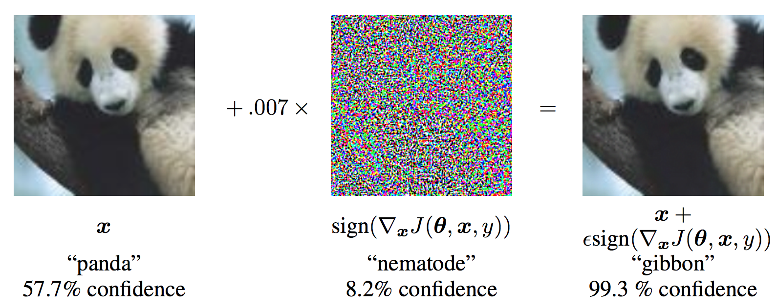
从该图可以发现，x 是原始的输入图像，并且可以正确的分类为 “Panda”，y 是其 ground truth label。对于 x，$\theta$ 代表模型的参数，$J(\theta, x, y)$ 是用于训练网络的损失。Attack 将该梯度反传给输入数据来计算。然后，调整微调输入的图像（例如，ϵ 或者 0.007 in the picture) in the direction (i.e. sign(∇xJ(θ,x,y))），使其可以最大化 loss。在此之后得到的 perturbed image x'，但是会被目标网络误分类为 “gibbon”，但是实际上看起来该图像仍然是一个 “Panda”。

 

来看下代码怎么写的。

 

from __future__ import print_function
import torch
import torch.nn as nn
import torch.nn.functional as F
import torch.optim as optim
from torchvision import datasets, transforms
import numpy as np
import matplotlib.pyplot as plt

 

Implementation: 

该教程的输入仅有三个：

epsilons --- List of epsilon values to use for the run. 

pretrained_model --- path to the pre-trained MNIST model which was trained with pytorch/examples/mnist. 

use_cuda ---- 是否利用 gpu。

 

epsilons = [0, .05, .1, .15, .2, .25, .3]
pretrained_model = "data/lenet_mnist_model.pth"
use_cuda=True

 

　　

 

Model Under Attack: 

 

# LeNet Model definition
class Net(nn.Module):
    def __init__(self):
        super(Net, self).__init__()
        self.conv1 = nn.Conv2d(1, 10, kernel_size=5)
        self.conv2 = nn.Conv2d(10, 20, kernel_size=5)
        self.conv2_drop = nn.Dropout2d()
        self.fc1 = nn.Linear(320, 50)
        self.fc2 = nn.Linear(50, 10)

    def forward(self, x):
        x = F.relu(F.max_pool2d(self.conv1(x), 2))
        x = F.relu(F.max_pool2d(self.conv2_drop(self.conv2(x)), 2))
        x = x.view(-1, 320)
        x = F.relu(self.fc1(x))
        x = F.dropout(x, training=self.training)
        x = self.fc2(x)
        return F.log_softmax(x, dim=1)

# MNIST Test dataset and dataloader declaration
test_loader = torch.utils.data.DataLoader(
    datasets.MNIST('../data', train=False, download=True, transform=transforms.Compose([
            transforms.ToTensor(),
            ])),
        batch_size=1, shuffle=True)

# Define what device we are using
print("CUDA Available: ",torch.cuda.is_available())
device = torch.device("cuda" if (use_cuda and torch.cuda.is_available()) else "cpu")

# Initialize the network
model = Net().to(device)

# Load the pretrained model
model.load_state_dict(torch.load(pretrained_model, map_location='cpu'))

# Set the model in evaluation mode. In this case this is for the Dropout layers
model.eval()

 

　　

FGSM Attack  

现在，我们可以定义function 通过修改原始的输入，来产生对抗样本。fgsm_attack 函数通过如下的方式来产生：

 

 

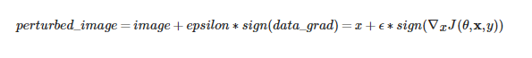
最终，为了保持 data 的范围，被修改后的数据被裁减为 [0, 1]：

 

# FGSM attack code
def fgsm_attack(image, epsilon, data_grad):
    # Collect the element-wise sign of the data gradient
    sign_data_grad = data_grad.sign()
    # Create the perturbed image by adjusting each pixel of the input image
    perturbed_image = image + epsilon*sign_data_grad
    # Adding clipping to maintain [0,1] range
    perturbed_image = torch.clamp(perturbed_image, 0, 1)
    # Return the perturbed image
    return perturbed_image

 

　　

 

Testing Function：

 

def test( model, device, test_loader, epsilon ):

    # Accuracy counter
    correct = 0
    adv_examples = []

    # Loop over all examples in test set
    for data, target in test_loader:

        # Send the data and label to the device
        data, target = data.to(device), target.to(device)

        # Set requires_grad attribute of tensor. Important for Attack
        data.requires_grad = True

        # Forward pass the data through the model
        output = model(data)
        init_pred = output.max(1, keepdim=True)[1] # get the index of the max log-probability

        # If the initial prediction is wrong, dont bother attacking, just move on
        if init_pred.item() != target.item():
            continue

        # Calculate the loss
        loss = F.nll_loss(output, target)

        # Zero all existing gradients
        model.zero_grad()

        # Calculate gradients of model in backward pass
        loss.backward()

        # Collect datagrad
        data_grad = data.grad.data

        # Call FGSM Attack
        perturbed_data = fgsm_attack(data, epsilon, data_grad)

        # Re-classify the perturbed image
        output = model(perturbed_data)

        # Check for success
        final_pred = output.max(1, keepdim=True)[1] # get the index of the max log-probability
        if final_pred.item() == target.item():
            correct += 1
            # Special case for saving 0 epsilon examples
            if (epsilon == 0) and (len(adv_examples) < 5):
                adv_ex = perturbed_data.squeeze().detach().cpu().numpy()
                adv_examples.append( (init_pred.item(), final_pred.item(), adv_ex) )
        else:
            # Save some adv examples for visualization later
            if len(adv_examples) < 5:
                adv_ex = perturbed_data.squeeze().detach().cpu().numpy()
                adv_examples.append( (init_pred.item(), final_pred.item(), adv_ex) )

    # Calculate final accuracy for this epsilon
    final_acc = correct/float(len(test_loader))
    print("Epsilon: {}\tTest Accuracy = {} / {} = {}".format(epsilon, correct, len(test_loader), final_acc))

    # Return the accuracy and an adversarial example
    return final_acc, adv_examples

 

　　

 

Run Attack：

accuracies = []
examples = []

# Run test for each epsilon
for eps in epsilons:
    acc, ex = test(model, device, test_loader, eps)
    accuracies.append(acc)
    examples.append(ex)

　　

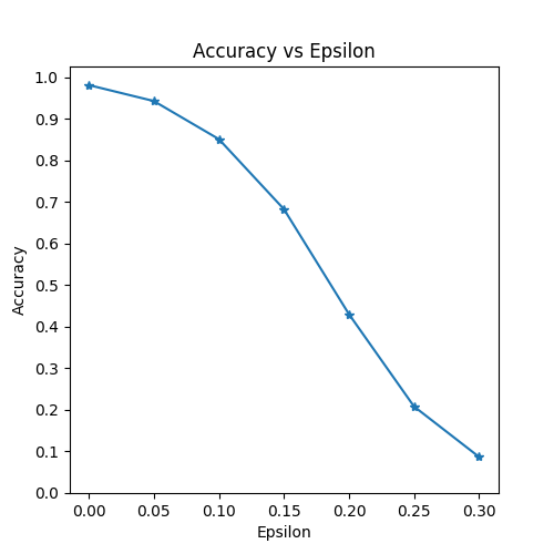
plt.figure(figsize=(5,5))
plt.plot(epsilons, accuracies, "*-")
plt.yticks(np.arange(0, 1.1, step=0.1))
plt.xticks(np.arange(0, .35, step=0.05))
plt.title("Accuracy vs Epsilon")
plt.xlabel("Epsilon")
plt.ylabel("Accuracy")
plt.show()

　　

 

 

 

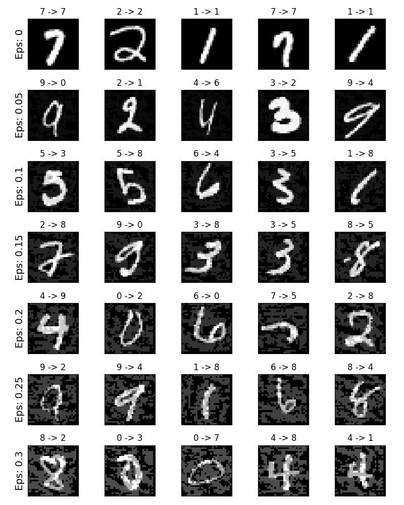
# Plot several examples of adversarial samples at each epsilon
cnt = 0
plt.figure(figsize=(8,10))
for i in range(len(epsilons)):
    for j in range(len(examples[i])):
        cnt += 1
        plt.subplot(len(epsilons),len(examples[0]),cnt)
        plt.xticks([], [])
        plt.yticks([], [])
        if j == 0:
            plt.ylabel("Eps: {}".format(epsilons[i]), fontsize=14)
        orig,adv,ex = examples[i][j]
        plt.title("{} -> {}".format(orig, adv))
        plt.imshow(ex, cmap="gray")
plt.tight_layout()
plt.show()