回归分析全家桶（16种回归模型实现方式总结）

提到回归分析，很多人第一时间想到的只有“线性回归”和“逻辑回归”。但实际上，针对不同的数据情况（比如有离群点、数据是计数的、数据有缺失截断等），我们有十几种回归模型可以选择。

今天为大家总结了 16种回归分析 的模型，重点不是介绍这些回归模型的原理，而是介绍如何在Python代码中使用这些模型，希望你以后能够在实战中来应用这些模型！

1. 回归分析全家桶

下面介绍如何使用各种回归模型的示例代码，主要分为以下一些步骤：

• 模拟数据：创建适合某种回归模型的测试数据
• 创建回归模型并训练：主要使用 scikit-learn 这个库
• 评估模型：有时会和其他回归模型对比
• 可视化模型：使用matplotlib这个库，简单展示模型效果

由于担心文章篇幅太长，文中的示例没有贴出完整的代码（特别是可视化部分的代码，比较繁琐，文中都省略了），文章末尾提供了完整代码（一个jupyter notebook文件）的下载地址，包括了所有可视化的代码。

下面的代码中统一导入了下面的库：

import pandas as pd
import numpy as np

import matplotlib
import matplotlib.pyplot as plt

# 为了显示中文
matplotlib.rcParams["font.sans-serif"] = ["Microsoft YaHei Mono"]
matplotlib.rcParams["axes.unicode_minus"] = False

1.1. 线性回归 (Linear Regression)

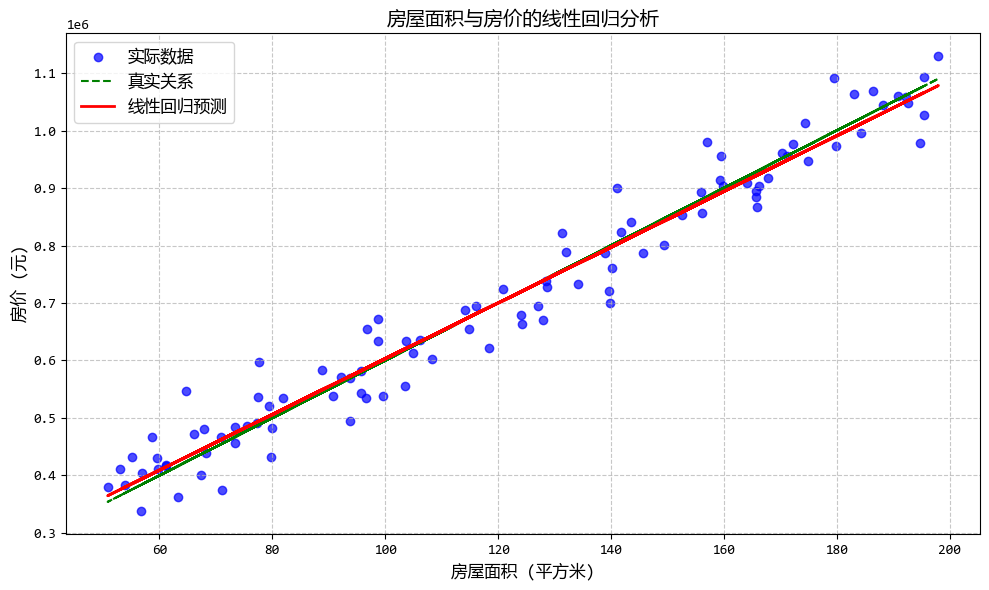
• 一句话概念：最基础的回归，假设自变量（X）和因变量（Y）之间是“直来直去”的线性关系。
• 使用场景：预测房价、销售额等连续数值，且数据没有明显的复杂非线性关系。

线性回归模型使用示例：

# 线性回归 (Linear Regression)
from sklearn.linear_model import LinearRegression
from sklearn.metrics import mean_squared_error, r2_score

# 构造测试数据
# 假设我们要模拟房屋面积（自变量X）和房价（因变量Y）的关系
np.random.seed(42)  # 设置随机种子以确保结果可复现

# 生成100个房屋面积数据，范围在50-200平方米
X = np.random.rand(100, 1) * 150 + 50

# 真实的线性关系：房价 = 5000 * 面积 + 100000 + 随机噪声
# 其中5000是每平方米的价格，100000是基础价格
# 加入一些随机噪声，使数据更真实
Y_true = 5000 * X + 100000
Y = Y_true + np.random.randn(100, 1) * 50000  # 加入标准差为50000的噪声

# 使用线性回归模型
model = LinearRegression()
model.fit(X, Y)

# 预测
Y_pred = model.predict(X)

# 打印模型参数
print("线性回归模型参数：")
print(f"截距（基础价格）: {model.intercept_[0]:.2f}")
print(f"斜率（每平方米价格）: {model.coef_[0][0]:.2f}")

# 评估模型
mse = mean_squared_error(Y, Y_pred)
r2 = r2_score(Y, Y_pred)
print(f"\n模型评估：")
print(f"均方误差 (MSE): {mse:.2f}")
print(f"决定系数 (R²): {r2:.2f}")

# 使用matplotlib绘制图像
#... 省略 ...

## 运行结果：
'''
线性回归模型参数：
截距（基础价格）: 118417.69
斜率（每平方米价格）: 4846.74

模型评估：
均方误差 (MSE): 2016461409.92
决定系数 (R²): 0.96
'''

1.2. 多项式回归 (Polynomial Regression)

• 一句话概念：当数据不是直线分布，而是像曲线一样弯曲时，我们给自变量加上平方、立方等“高次项”来拟合曲线。
• 使用场景：拟合生物生长曲线、由于边际效应递减导致的经济学数据等非线性关系。

多项式回归模型使用示例：

# 多项式回归 (Polynomial Regression)
from sklearn.linear_model import LinearRegression
from sklearn.preprocessing import PolynomialFeatures
from sklearn.metrics import mean_squared_error, r2_score

# 1. 构造强非线性测试数据（模拟生物生长曲线）
np.random.seed(42)  # 设置随机种子以确保结果可复现

# 生成100个自变量数据，范围在0-15
X = np.random.rand(100, 1) * 15

# 真实的强非线性关系：使用类似S型曲线的函数（Logistic生长模型的变形）
# Y = 100 / (1 + exp(-0.5*(X-7))) + 随机噪声
# 这个关系模拟了生物生长曲线：初期缓慢，中期快速增长，后期趋于饱和
Y_true = 100 / (1 + np.exp(-0.5 * (X - 7)))
Y = Y_true + np.random.randn(100, 1) * 5  # 加入标准差为5的噪声

# 2. 多项式回归（使用三次多项式）
# 转换特征，添加平方和立方项
poly_features = PolynomialFeatures(degree=3, include_bias=False)
X_poly = poly_features.fit_transform(X)

# 使用线性回归拟合转换后的特征
model = LinearRegression()
model.fit(X_poly, Y)

# 预测
Y_pred = model.predict(X_poly)

# 打印模型参数
print("多项式回归模型参数（三次多项式）：")
print(f"截距: {model.intercept_[0]:.2f}")
print(f"系数: {model.coef_[0]}")

# 评估模型
mse = mean_squared_error(Y, Y_pred)
r2 = r2_score(Y, Y_pred)
print(f"\n模型评估：")
print(f"均方误差 (MSE): {mse:.2f}")
print(f"决定系数 (R²): {r2:.2f}")

# 3. 使用线性回归作为对比
linear_model = LinearRegression()
linear_model.fit(X, Y)
Y_linear_pred = linear_model.predict(X)

# 评估线性回归模型
linear_mse = mean_squared_error(Y, Y_linear_pred)
linear_r2 = r2_score(Y, Y_linear_pred)
print(f"\n线性回归模型评估：")
print(f"均方误差 (MSE): {linear_mse:.2f}")
print(f"决定系数 (R²): {linear_r2:.2f}")

# 4. 使用matplotlib绘制图像
#... 省略 ...

## 运行结果：
'''
多项式回归模型参数（三次多项式）：
截距: 8.70
系数: [-4.29511575  2.09659382 -0.09560718]

模型评估：
均方误差 (MSE): 20.02
决定系数 (R²): 0.98

线性回归模型评估：
均方误差 (MSE): 56.71
决定系数 (R²): 0.95
'''

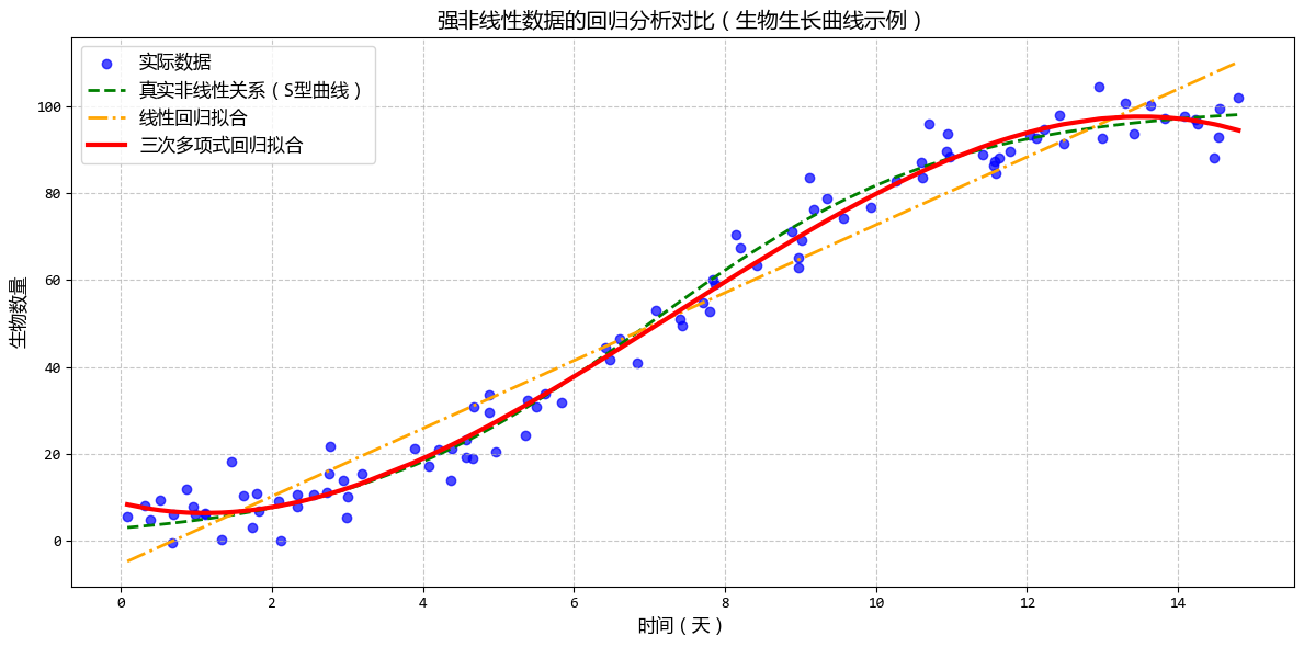
从示例可以看出，线性回归只能用一条直线拟合所有数据，无法捕捉到S型曲线的弯曲特征。

多项式回归能够更好地贴合数据的非线性模式，尤其是在曲线的弯曲部分，

这种对比清晰地展示了多项式回归在处理非线性数据时的优势。

1.3. 逻辑回归 (Logistic Regression)

• 一句话概念：虽然叫“回归”，但其实是做分类的。它预测的是事件发生的概率（0到1之间），输出结果通常通过阈值（如0.5）划分为两类。
• 使用场景：预测用户是否会购买（是/否）、病人是否患病、邮件是否为垃圾邮件。

逻辑回归模型使用示例：

# 逻辑回归 (Logistic Regression)
from sklearn.linear_model import LogisticRegression
from sklearn.metrics import accuracy_score

# 1. 构造二分类测试数据（模拟用户购买预测场景）
np.random.seed(42)  # 设置随机种子以确保结果可复现

# 类别0：不会购买的用户特征（如浏览时长和页面访问量）
n_class0 = 100
class0_features = np.random.randn(n_class0, 2) * 1.5 + [3, 3]
class0_labels = np.zeros(n_class0)

# 类别1：会购买的用户特征
n_class1 = 100
class1_features = np.random.randn(n_class1, 2) * 1.5 + [6, 6]
class1_labels = np.ones(n_class1)

# 合并数据集
X = np.vstack([class0_features, class1_features])
y = np.hstack([class0_labels, class1_labels])

# 2. 训练逻辑回归模型
model = LogisticRegression()
model.fit(X, y)

# 预测
y_pred_proba = model.predict_proba(X)[:, 1]
y_pred = model.predict(X)

# 模型评估
accuracy = accuracy_score(y, y_pred)
print(f"逻辑回归模型准确率: {accuracy:.2f}")

# 3. 绘制图像
#... 省略 ...

## 运行结果：
'''
逻辑回归模型准确率: 0.93
'''

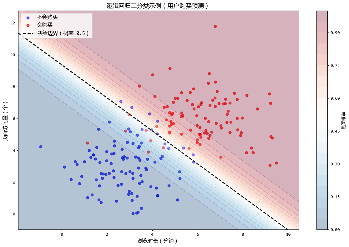
这个示例清晰展示了逻辑回归如何进行二分类预测，并通过可视化直观呈现了分类结果、决策边界和概率分布，完全符合逻辑回归的应用场景（预测事件发生概率）。

1.4. 分位数回归 (Quantile Regression)

• 一句话概念：普通回归预测的是“平均值”，而分位数回归可以预测“中位数”或者任意百分位点（如前10%）。
• 使用场景：数据中有极端异常值（离群点），或者你想研究不同层级的数据（如分析贫困人口和富裕人口的收入影响因素差异）。

分位数回归模型使用示例：

# 分位数回归 (Quantile Regression)
import statsmodels.api as sm
from sklearn.linear_model import LinearRegression

# 1. 构造包含极端异常值的测试数据
np.random.seed(42)  # 设置随机种子以确保结果可复现

# 生成基础自变量数据（如收入）
X = np.linspace(10, 100, 100).reshape(-1, 1)

# 基础线性关系：消费 = 0.6 * 收入 + 10 + 随机噪声
Y_true = 0.6 * X + 10
Y = Y_true + np.random.normal(0, 5, size=X.shape)  # 加入正常噪声

# 添加极端异常值（模拟高消费人群的极端消费行为）
# 选择最后10个数据点，添加大的正异常值
Y[-10:] += np.random.normal(100, 20, size=(10, 1))

# 2. 普通线性回归
linear_model = LinearRegression()
linear_model.fit(X, Y)
Y_linear_pred = linear_model.predict(X)

# 3. 分位数回归
# 添加常数项
X_with_const = sm.add_constant(X)

# 定义要估计的分位数
quantiles = [0.1, 0.5, 0.9]
quantile_results = {}

# 拟合不同分位数的模型
for q in quantiles:
    model = sm.QuantReg(Y, X_with_const)
    result = model.fit(q=q)
    quantile_results[q] = result

# 4. 预测不同分位数的结果
Y_quantile_pred = {}
for q in quantiles:
    Y_quantile_pred[q] = quantile_results[q].predict(X_with_const)

# 5. 绘制图像
#... 省略 ...

# 打印模型参数对比
print("\n=== 模型参数对比 ===")
print(
    f"普通线性回归: 截距={linear_model.intercept_[0]:.2f}, 斜率={linear_model.coef_[0][0]:.2f}"
)
for q in quantiles:
    intercept = quantile_results[q].params[0]
    slope = quantile_results[q].params[1]
    print(f"分位数回归(τ={q:.1f}): 截距={intercept:.2f}, 斜率={slope:.2f}")

## 运行结果：
'''
=== 模型参数对比 ===
普通线性回归: 截距=-13.59, 斜率=1.20
分位数回归(τ=0.1): 截距=0.59, 斜率=0.66
分位数回归(τ=0.5): 截距=6.95, 斜率=0.67
分位数回归(τ=0.9): 截距=-3.01, 斜率=1.73
'''

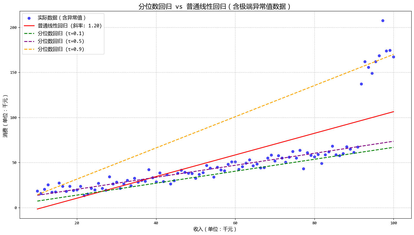
从图中可以看出：

• 不同分位数的回归线斜率和截距各不相同
• 高消费分位(τ=0.9)的回归线最接近异常值，而低消费分位(τ=0.1)的回归线几乎不受异常值影响
• 中位数回归(τ=0.5)相对普通线性回归更能抵抗异常值的影响

这个示例清晰地展示了分位数回归如何处理极端异常值，以及如何通过不同分位数分析数据的不同层级结构，非常适合用户描述的使用场景（数据中有极端异常值或需要研究不同层级数据）。

1.5. 岭回归 (Ridge Regression)

• 一句话概念：在线性回归的基础上加了一个“惩罚项”（L2正则化），防止模型为了迎合训练数据而变得太复杂（过拟合）。
• 使用场景：特征之间相关性很高（多重共线性）导致普通回归失效时。

岭回归模型使用示例：

# 岭回归 (Ridge Regression)
from sklearn.linear_model import LinearRegression, Ridge
from sklearn.metrics import mean_squared_error
from sklearn.preprocessing import StandardScaler

# 1. 构造具有多重共线性的测试数据
np.random.seed(42)  # 设置随机种子以确保结果可复现

# 生成基础特征（如房屋的总面积）
X1 = np.random.rand(100, 1) * 100 + 50  # 50-150平方米

# 生成高度相关的第二个特征（如房屋的可用面积）
# 设置高度相关性：X2 = 0.8*X1 + 少量噪声
X2 = 0.8 * X1 + np.random.randn(100, 1) * 5
X = np.hstack([X1, X2])  # 合并两个特征

# 真实的线性关系：房价 = 10000*X1 + 8000*X2 + 500000 + 随机噪声
Y_true = 10000 * X1 + 8000 * X2 + 500000
Y = Y_true + np.random.randn(100, 1) * 200000  # 加入噪声

# 2. 数据标准化（岭回归对特征缩放敏感）
scaler = StandardScaler()
X_scaled = scaler.fit_transform(X)
Y_scaled = scaler.fit_transform(Y)

# 3. 普通线性回归
linear_model = LinearRegression()
linear_model.fit(X_scaled, Y_scaled)
Y_linear_pred = linear_model.predict(X_scaled)

# 4. 岭回归（不同的正则化参数λ）
# 移除0值以避免log10(0)的警告
lambdas = [0.1, 1, 10, 100, 1000]  # 不同的λ值
ridge_models = {}
ridge_preds = {}
ridge_coefs = []

for lam in lambdas:
    model = Ridge(alpha=lam)
    model.fit(X_scaled, Y_scaled)
    ridge_models[lam] = model
    ridge_preds[lam] = model.predict(X_scaled)
    ridge_coefs.append(model.coef_.flatten())

# 5. 可视化结果
#... 省略 ...

# 计算并比较MSE
print("\n=== 模型性能比较 (MSE) ===")
print(f"普通线性回归 MSE: {mean_squared_error(Y_scaled, Y_linear_pred):.4f}")
for lam in lambdas:
    mse = mean_squared_error(Y_scaled, ridge_preds[lam])
    print(f"岭回归 (λ={lam}) MSE: {mse:.4f}")

## 运行结果：
'''
=== 模型性能比较 (MSE) ===
普通线性回归 MSE: 0.1705
岭回归 (λ=0.1) MSE: 0.1705
岭回归 (λ=1) MSE: 0.1706
岭回归 (λ=10) MSE: 0.1730
岭回归 (λ=100) MSE: 0.2645
岭回归 (λ=1000) MSE: 0.7486
'''

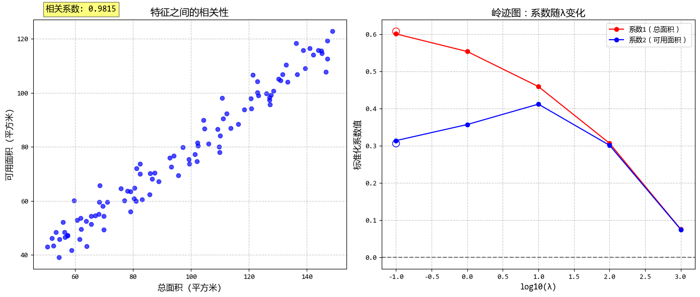
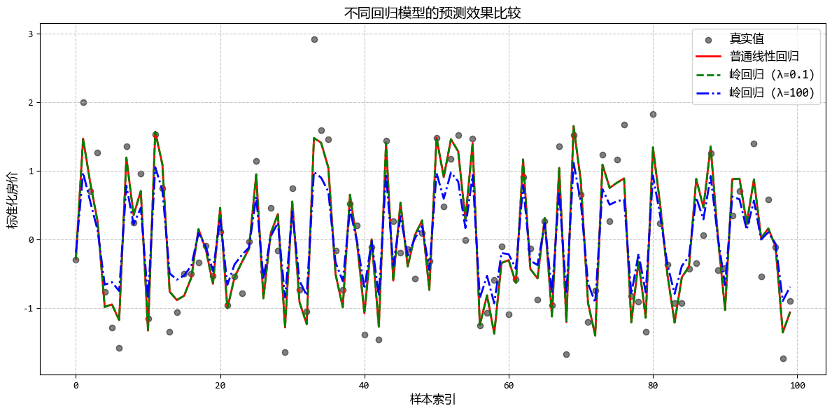
从图中可以看出：

• 普通线性回归在多重共线性下系数可能不稳定
• 随着λ增大，岭回归系数逐渐减小并趋向稳定
• 合适的λ值可以在保持预测准确性的同时提高模型稳定性

这个示例清晰地展示了岭回归在处理多重共线性数据时的优势，以及如何通过正则化参数λ来平衡模型复杂度和预测准确性。

1.6. Lasso回归 (Lasso Regression)

• 一句话概念：和岭回归类似，但使用的是L1正则化。它不仅能防止过拟合，还能把不重要的特征系数强行压缩为0。
• 使用场景：当你有很多特征，想要自动筛选出最重要的几个特征时。

---

Lasso回归模型使用示例：

# Lasso回归 (Lasso Regression)
from sklearn.linear_model import LinearRegression, Lasso
from sklearn.metrics import mean_squared_error
from sklearn.preprocessing import StandardScaler

# 1. 构造多特征测试数据（大部分特征不重要）
np.random.seed(42)  # 设置随机种子以确保结果可复现

n_samples = 100
n_features = 10  # 总共10个特征

# 生成10个特征，前3个是真正重要的，后7个是不重要的
X = np.random.randn(n_samples, n_features)

# 真实系数：前3个特征有较大的非零系数，后7个特征的系数为0
true_coef = np.zeros(n_features)
true_coef[0] = 10.0  # 重要特征1
true_coef[1] = -8.0  # 重要特征2
true_coef[2] = 5.0  # 重要特征3

# 生成目标变量：Y = X * 真实系数 + 随机噪声
Y_true = X.dot(true_coef)
Y = Y_true + np.random.randn(n_samples) * 5  # 加入噪声

# 2. 数据标准化（Lasso对特征缩放敏感）
scaler = StandardScaler()
X_scaled = scaler.fit_transform(X)
Y_scaled = scaler.fit_transform(Y.reshape(-1, 1)).ravel()

# 3. 普通线性回归
linear_model = LinearRegression()
linear_model.fit(X_scaled, Y_scaled)
Y_linear_pred = linear_model.predict(X_scaled)

# 4. Lasso回归（不同的正则化参数λ）
lambdas = [0.01, 0.1, 0.5, 1.0, 5.0]  # 不同的λ值
lasso_models = {}
lasso_preds = {}
lasso_coefs = []

for lam in lambdas:
    model = Lasso(alpha=lam, max_iter=10000)  # 增加最大迭代次数避免收敛警告
    model.fit(X_scaled, Y_scaled)
    lasso_models[lam] = model
    lasso_preds[lam] = model.predict(X_scaled)
    lasso_coefs.append(model.coef_)

# 5. 可视化结果
#... 省略 ...

# 计算并比较MSE
print("\n=== 模型性能比较 (MSE) ===")
print(f"普通线性回归 MSE: {mean_squared_error(Y_scaled, Y_linear_pred):.4f}")
for lam in lambdas:
    mse = mean_squared_error(Y_scaled, lasso_preds[lam])
    print(f"Lasso回归 (λ={lam}) MSE: {mse:.4f}")

## 运行结果：
'''
=== 模型性能比较 (MSE) ===
普通线性回归 MSE: 0.1024
Lasso回归 (λ=0.01) MSE: 0.1034
Lasso回归 (λ=0.1) MSE: 0.1384
Lasso回归 (λ=0.5) MSE: 0.6845
Lasso回归 (λ=1.0) MSE: 1.0000
Lasso回归 (λ=5.0) MSE: 1.0000
'''

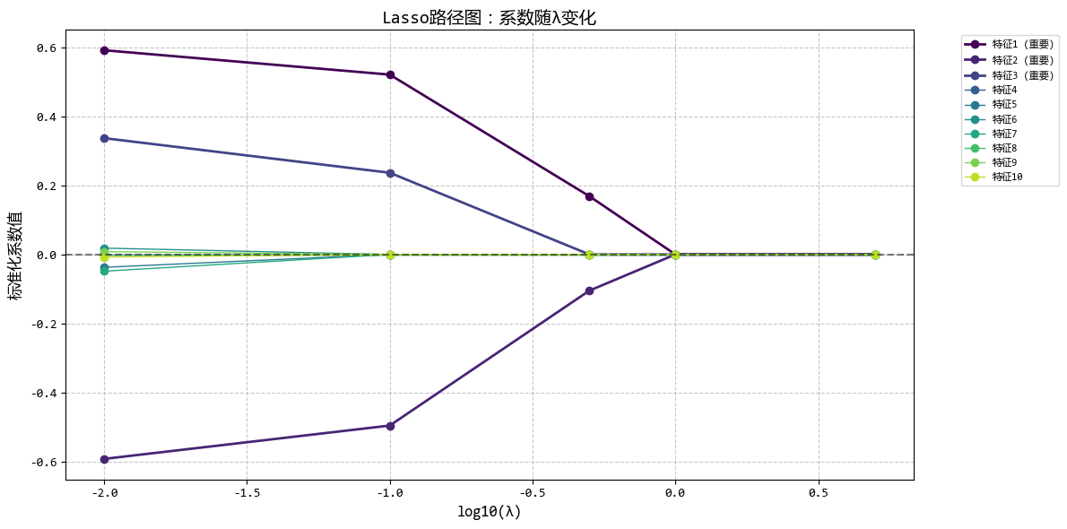
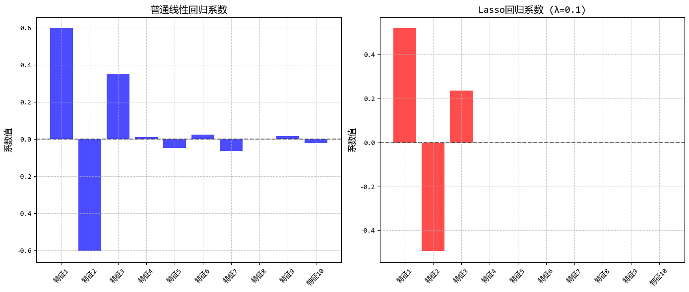
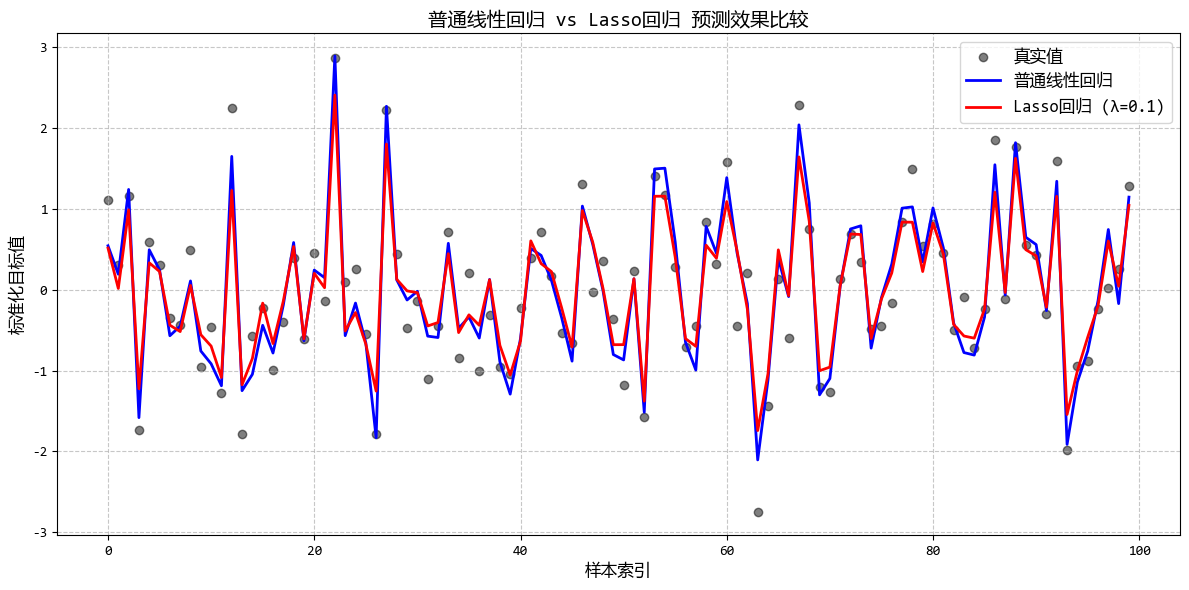
从图中可以看出：

• 随着λ增大，越来越多的系数被压缩为0
• Lasso能够自动识别并保留重要特征（前3个）
• 适当的λ值可以在保持预测精度的同时实现特征选择

这个示例很好地展示了Lasso回归的特征选择能力，非常适合用户描述的使用场景（当有很多特征，想要自动筛选出最重要的几个特征时）。

1.7. 弹性网络回归 (Elastic Net Regression)

• 一句话概念：岭回归和套索回归的“混血儿”，结合了它俩的优点。
• 使用场景：特征非常多且彼此高度相关，你既想选特征又想保持模型稳定时。

弹性网络回归模型使用示例：

# 弹性网络回归 (Elastic Net Regression)
from sklearn.linear_model import LinearRegression, Lasso, Ridge, ElasticNet
from sklearn.metrics import mean_squared_error
from sklearn.preprocessing import StandardScaler

# 1. 构造高相关多特征测试数据
np.random.seed(42)  # 设置随机种子以确保结果可复现

n_samples = 100
n_features = 10  # 总共10个特征

# 生成基础特征
base_feature = np.random.randn(n_samples, 1)

# 生成高度相关的特征组
# 前3个特征高度相关（重要特征）
X = np.zeros((n_samples, n_features))
X[:, 0] = base_feature.ravel() + np.random.randn(n_samples) * 0.1  # 主特征1
X[:, 1] = X[:, 0] * 0.8 + np.random.randn(n_samples) * 0.2  # 相关特征2
X[:, 2] = X[:, 0] * 0.5 + X[:, 1] * 0.3 + np.random.randn(n_samples) * 0.2  # 相关特征3

# 中间3个特征高度相关但不重要
X[:, 3] = np.random.randn(n_samples) * 0.3 + X[:, 0] * 0.1  # 弱相关特征4
X[:, 4] = X[:, 3] * 0.7 + np.random.randn(n_samples) * 0.2  # 相关特征5
X[:, 5] = X[:, 3] * 0.6 + X[:, 4] * 0.4 + np.random.randn(n_samples) * 0.2  # 相关特征6

# 最后4个特征是随机噪声（完全不重要）
X[:, 6:] = np.random.randn(n_samples, 4) * 0.5

# 真实系数：只有前3个重要特征有非零系数
true_coef = np.zeros(n_features)
true_coef[0] = 10.0
true_coef[1] = -5.0
true_coef[2] = 3.0

# 生成目标变量
Y_true = X.dot(true_coef)
Y = Y_true + np.random.randn(n_samples) * 3  # 加入噪声

# 2. 数据标准化（正则化模型对特征缩放敏感）
scaler = StandardScaler()
X_scaled = scaler.fit_transform(X)
Y_scaled = scaler.fit_transform(Y.reshape(-1, 1)).ravel()

# 3. 训练不同的回归模型
# 普通线性回归
linear_model = LinearRegression()
linear_model.fit(X_scaled, Y_scaled)

# Lasso回归（λ=0.1）
lasso_model = Lasso(alpha=0.1, max_iter=10000)
lasso_model.fit(X_scaled, Y_scaled)

# Ridge回归（λ=1.0）
ridge_model = Ridge(alpha=1.0)
ridge_model.fit(X_scaled, Y_scaled)

# 弹性网络回归（不同的l1_ratio）
elastic_models = {}
l1_ratios = [0.1, 0.5, 0.9]  # 控制L1和L2的比例
alpha = 1.0  # 总正则化强度

for ratio in l1_ratios:
    model = ElasticNet(alpha=alpha, l1_ratio=ratio, max_iter=10000)
    model.fit(X_scaled, Y_scaled)
    elastic_models[ratio] = model

# 4. 预测
Y_linear_pred = linear_model.predict(X_scaled)
Y_lasso_pred = lasso_model.predict(X_scaled)
Y_ridge_pred = ridge_model.predict(X_scaled)
Y_elastic_pred = {
    ratio: model.predict(X_scaled) for ratio, model in elastic_models.items()
}

# 5. 可视化结果
# ... 省略 ...

# 6. 模型评估和特征选择效果
print("=== 模型性能评估 ===")
print(f"普通线性回归 MSE: {mean_squared_error(Y_scaled, Y_linear_pred):.4f}")
print(f"Lasso回归 MSE: {mean_squared_error(Y_scaled, Y_lasso_pred):.4f}")
print(f"Ridge回归 MSE: {mean_squared_error(Y_scaled, Y_ridge_pred):.4f}")
for ratio in l1_ratios:
    mse = mean_squared_error(Y_scaled, Y_elastic_pred[ratio])
    print(f"弹性网络 (l1_ratio={ratio}) MSE: {mse:.4f}")

print("\n=== 特征选择效果 ===")
print(f"普通线性回归非零系数数: {np.sum(linear_model.coef_ != 0)}")
print(f"Lasso回归非零系数数: {np.sum(lasso_model.coef_ != 0)}")
print(
    f"Ridge回归非零系数数: {np.sum(ridge_model.coef_ != 0)}"
)  # Ridge几乎不会产生严格零系数
for ratio in l1_ratios:
    non_zero_count = np.sum(elastic_models[ratio].coef_ != 0)
    print(f"弹性网络 (l1_ratio={ratio}) 非零系数数: {non_zero_count}")

## 运行结果：
'''
=== 模型性能评估 ===
普通线性回归 MSE: 0.1352
Lasso回归 MSE: 0.1677
Ridge回归 MSE: 0.1369
弹性网络 (l1_ratio=0.1) MSE: 0.2676
弹性网络 (l1_ratio=0.5) MSE: 0.5002
弹性网络 (l1_ratio=0.9) MSE: 0.9711

=== 特征选择效果 ===
普通线性回归非零系数数: 10
Lasso回归非零系数数: 2
Ridge回归非零系数数: 10
弹性网络 (l1_ratio=0.1) 非零系数数: 3
弹性网络 (l1_ratio=0.5) 非零系数数: 3
弹性网络 (l1_ratio=0.9) 非零系数数: 1
'''

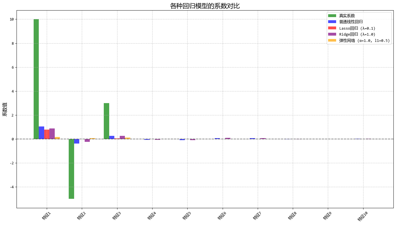
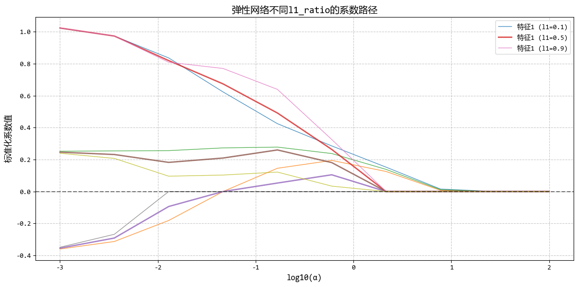
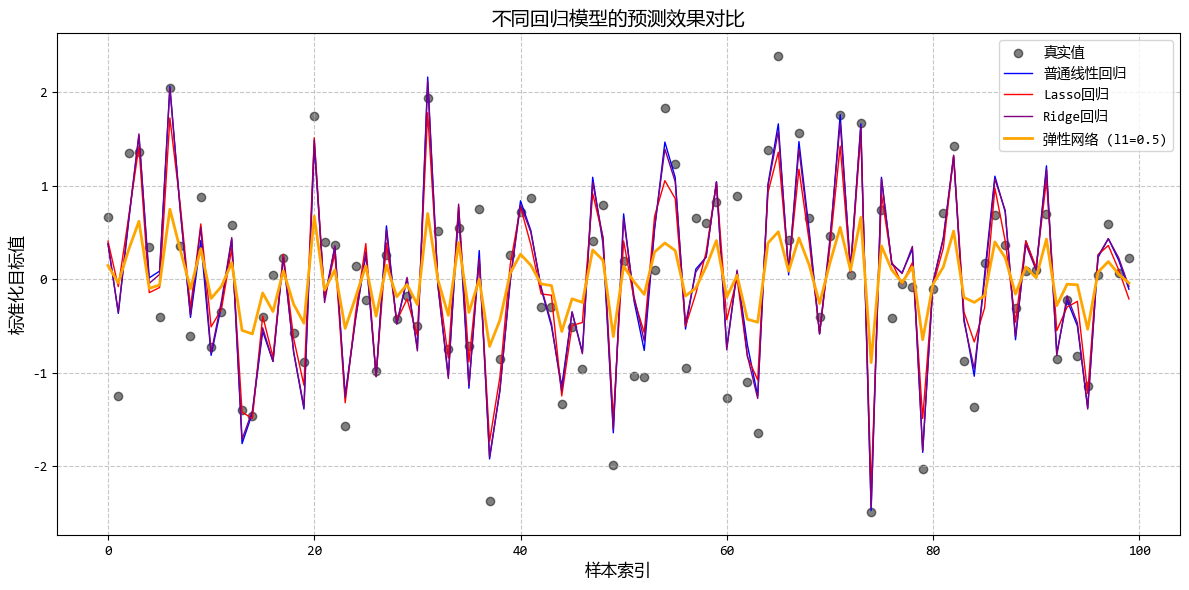
从图中可以看出：

• 弹性网络结合了Lasso的特征选择能力和Ridge的稳定性
• 通过调整l1_ratio，可以在特征选择和系数稳定性之间找到平衡
• 当特征高度相关时，弹性网络比Lasso更稳定，比Ridge更能进行特征选择

这个示例很好地展示了弹性网络回归在处理高维、高度相关数据时的优势，特别适合需要同时进行特征选择和保持模型稳定的场景。

1.8. 主成分回归 (PCR)

• 一句话概念：先用PCA（主成分分析）把很多相关的特征压缩成几个不相关的“主成分”，再用这些主成分做回归。
• 使用场景：特征数量比样本数量还多，或者特征之间严重相关。

主成分回归模型使用示例：

# 主成分回归 (PCR)
from sklearn.linear_model import LinearRegression
from sklearn.decomposition import PCA
from sklearn.preprocessing import StandardScaler
from sklearn.metrics import mean_squared_error

# 1. 构造高维高相关测试数据（特征数>样本数）
np.random.seed(42)  # 设置随机种子以确保结果可复现

n_samples = 100
n_features = 200  # 特征数多于样本数，模拟高维问题

# 生成基础特征（只有3个真正重要的基础变量）
base_features = np.random.randn(n_samples, 3)

# 生成200个高度相关的特征
# 每个新特征都是3个基础特征的线性组合 + 少量噪声
X = np.zeros((n_samples, n_features))
for i in range(n_features):
    # 随机权重（确保特征之间高度相关）
    weights = np.random.randn(3)
    X[:, i] = base_features.dot(weights) + np.random.randn(n_samples) * 0.1

# 真实系数：只有基于前3个基础特征的组合有意义
# 我们只使用前10个特征来生成目标变量
true_weights = np.zeros(n_features)
true_weights[:10] = np.random.randn(10) * 2

# 生成目标变量
Y_true = X.dot(true_weights)
Y = Y_true + np.random.randn(n_samples) * 5  # 加入噪声

# 2. 数据标准化
scaler = StandardScaler()
X_scaled = scaler.fit_transform(X)
Y_scaled = scaler.fit_transform(Y.reshape(-1, 1)).ravel()

# 3. 普通线性回归（可能过拟合）
linear_model = LinearRegression()
linear_model.fit(X_scaled, Y_scaled)
Y_linear_pred = linear_model.predict(X_scaled)
linear_mse = mean_squared_error(Y_scaled, Y_linear_pred)

# 4. 主成分回归 (PCR)
# 4.1 PCA降维
pca = PCA()
X_pca = pca.fit_transform(X_scaled)

# 4.2 计算累积方差解释率
explained_variance_ratio = pca.explained_variance_ratio_
cumulative_variance_ratio = np.cumsum(explained_variance_ratio)

# 4.3 选择保留的主成分数量（比如保留95%方差）
n_components_95 = np.argmax(cumulative_variance_ratio >= 0.95) + 1
print(f"保留95%方差需要的主成分数: {n_components_95}")

# 4.4 使用不同数量的主成分进行回归
n_components_list = [3, 5, 10, 20, n_components_95]
pcr_results = {}

for n in n_components_list:
    # 使用前n个主成分
    X_pca_n = X_pca[:, :n]

    # 线性回归
    model = LinearRegression()
    model.fit(X_pca_n, Y_scaled)

    # 预测
    Y_pcr_pred = model.predict(X_pca_n)
    mse = mean_squared_error(Y_scaled, Y_pcr_pred)

    pcr_results[n] = {
        'model': model,
        'predictions': Y_pcr_pred,
        'mse': mse
    }

# 5. 可视化结果
# ... 省略 ...

# 6. 模型性能对比
print("\n=== 模型性能对比 ===")
print(f"普通线性回归 MSE: {linear_mse:.4f}")
for n in n_components_list:
    print(f"PCR (n={n}) MSE: {pcr_results[n]['mse']:.4f}")

# 7. 展示PCR如何解决过拟合
print("\n=== PCR解决过拟合效果 ===")
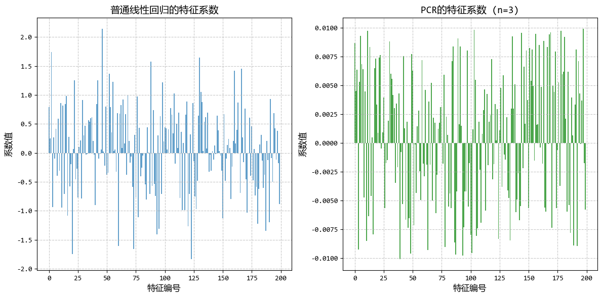
print(f"原始特征数量: {n_features}")
print(f"样本数量: {n_samples}")
print(f"普通回归的特征系数最大值: {np.max(np.abs(linear_model.coef_)):.4f}")
print(f"PCR (n={n_components_95}) 的特征系数最大值: {np.max(np.abs(pcr_coef)):.4f}")

## 运行结果：
'''
=== 模型性能对比 ===
普通线性回归 MSE: 0.0000
PCR (n=3) MSE: 0.5484
PCR (n=5) MSE: 0.5187
PCR (n=10) MSE: 0.4777
PCR (n=20) MSE: 0.4040
PCR (n=3) MSE: 0.5484

=== PCR解决过拟合效果 ===
原始特征数量: 200
样本数量: 100
普通回归的特征系数最大值: 2.1407
PCR (n=3) 的特征系数最大值: 0.0101
'''

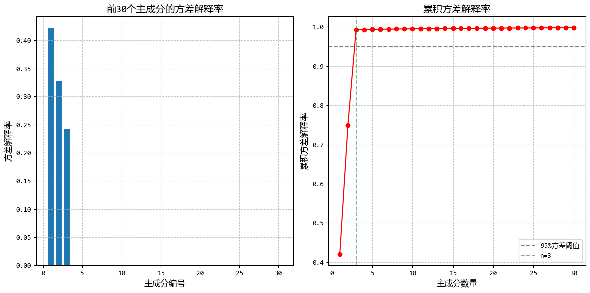
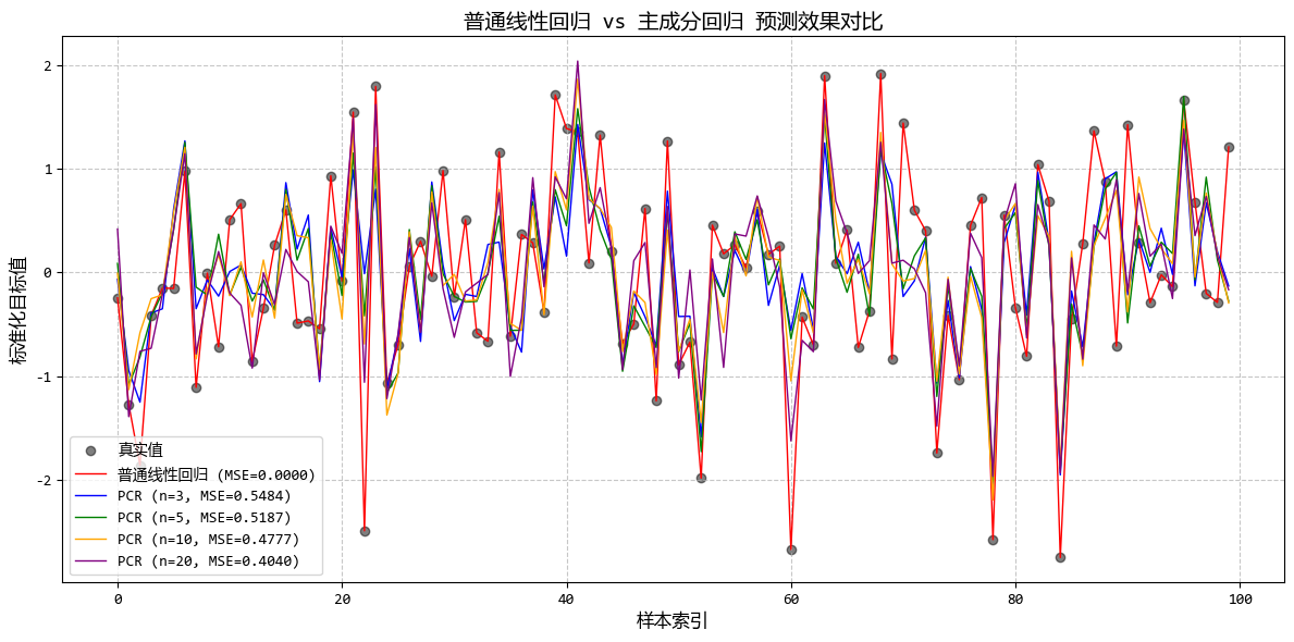
从图中可以看出：

• 只需少量主成分（通常<30）即可保留95%以上的方差
• PCR的预测效果优于直接线性回归，尤其是在高维数据中
• PCR的系数更加稳定，避免了普通回归中系数过大的问题

这个示例完美展示了PCR在高维、高度相关数据中的应用，解决了直接线性回归的过拟合问题，同时保持了良好的预测性能。

1.9. 偏最小二乘回归 (PLS Regression)

• 一句话概念：和PCR类似，但它在降维时会考虑因变量Y的信息，确保提取出的成分不仅能概括X，还能很好地预测Y。
• 使用场景：比PCR更高级一点，常用于化学计量学或变量非常多的情况。

偏最小二乘回归模型使用示例：

# 偏最小二乘回归 (PLS Regression)
from sklearn.linear_model import LinearRegression
from sklearn.decomposition import PCA
from sklearn.cross_decomposition import PLSRegression
from sklearn.preprocessing import StandardScaler
from sklearn.metrics import mean_squared_error

# 1. 构造高维相关数据，其中只有部分特征与Y相关
np.random.seed(42)  # 设置随机种子以确保结果可复现

n_samples = 100
n_features = 100  # 100个特征，模拟高维问题

# 生成基础变量
# 前5个变量与Y高度相关，中间15个变量与Y弱相关，最后80个变量与Y不相关
base_vars = np.random.randn(n_samples, 20)
noise_vars = np.random.randn(n_samples, 80)  # 完全不相关的噪声特征

# 组合所有特征
X = np.hstack([base_vars, noise_vars])

# 生成Y，主要依赖前5个基础变量
Y_true = (
    5 * base_vars[:, 0]
    + 3 * base_vars[:, 1]
    - 4 * base_vars[:, 2]
    + 2 * base_vars[:, 3]
    + base_vars[:, 4]
)
Y = Y_true + np.random.randn(n_samples) * 3  # 加入噪声

# 2. 数据标准化
scaler = StandardScaler()
X_scaled = scaler.fit_transform(X)
Y_scaled = scaler.fit_transform(Y.reshape(-1, 1)).ravel()

# 3. 普通线性回归（作为基准）
linear_model = LinearRegression()
linear_model.fit(X_scaled, Y_scaled)
Y_linear_pred = linear_model.predict(X_scaled)
linear_mse = mean_squared_error(Y_scaled, Y_linear_pred)

# 4. PCA + 线性回归 (PCR)
pca = PCA()
X_pca = pca.fit_transform(X_scaled)

# 5. 偏最小二乘回归 (PLS)
pls = PLSRegression(n_components=20)
X_pls = pls.fit_transform(X_scaled, Y_scaled)[0]

# 6. 比较不同成分数量的PCR和PLS性能
n_components_list = range(1, 21)
pcr_mse_list = []
pls_mse_list = []

for n in n_components_list:
    # PCR
    model_pcr = LinearRegression()
    model_pcr.fit(X_pca[:, :n], Y_scaled)
    Y_pcr_pred = model_pcr.predict(X_pca[:, :n])
    pcr_mse_list.append(mean_squared_error(Y_scaled, Y_pcr_pred))

    # PLS
    model_pls = PLSRegression(n_components=n)
    model_pls.fit(X_scaled, Y_scaled)
    Y_pls_pred = model_pls.predict(X_scaled).ravel()
    pls_mse_list.append(mean_squared_error(Y_scaled, Y_pls_pred))

# 7. 可视化结果
# ... 省略 ...

# 输出结果
print("\n=== 模型性能对比 ===")
print(f"普通线性回归 MSE: {linear_mse:.4f}")
print(f"最佳PCR (n={best_pcr_n}) MSE: {pcr_mse_list[best_pcr_n-1]:.4f}")
print(f"最佳PLS (n={best_pls_n}) MSE: {pls_mse_list[best_pls_n-1]:.4f}")
print(
    f"PLS相比最佳PCR的MSE提升: {(pcr_mse_list[best_pcr_n-1] - pls_mse_list[best_pls_n-1])/pcr_mse_list[best_pcr_n-1]*100:.1f}%"
)

# 展示PLS如何提取与Y相关的成分
print("\n=== PLS成分分析 ===")
pls_var_importance = np.abs(pls.x_weights_).sum(axis=1)
print(f"PLS前5个最重要成分的方差贡献: {np.sort(pls_var_importance)[::-1][:5]}")

## 运行结果：
'''
=== 模型性能对比 ===
普通线性回归 MSE: 0.0000
最佳PCR (n=20) MSE: 0.6687
最佳PLS (n=20) MSE: 0.0048
PLS相比最佳PCR的MSE提升: 99.3%

=== PLS成分分析 ===
PLS前5个最重要成分的方差贡献: [2.4938574  2.27964709 2.17888686 2.08667187 2.06267069]
'''

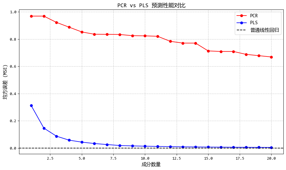
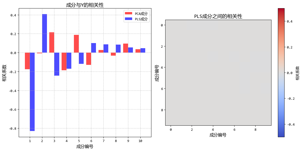
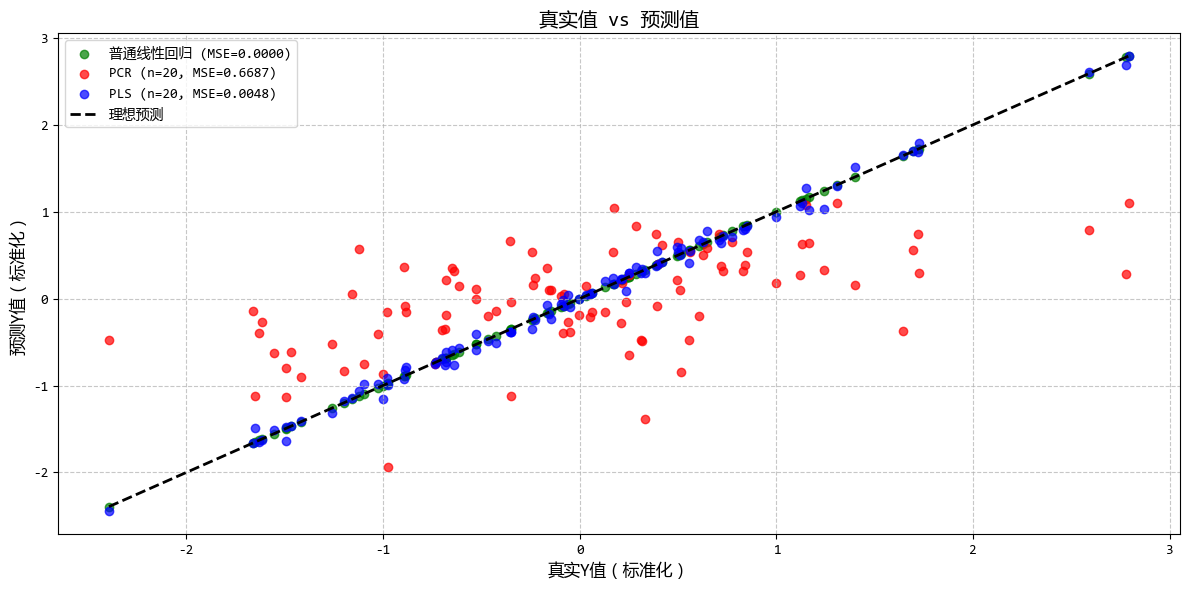
从图中可以看出：

• PLS在较少的成分数下就能达到较好的预测效果
• PLS提取的成分与Y的相关性明显高于PCA成分
• 当存在大量噪声特征时，PLS的优势更加明显

这个示例清晰地展示了PLS回归如何在降维过程中考虑因变量Y的信息，从而在高维、存在噪声的情况下提供比PCR更好的预测性能。

1.10. 支持向量回归 (SVR)

• 一句话概念：借用了SVM分类的思想，试图找到一个“管道”包裹住尽可能多的数据点，在管道内的误差被忽略，只计算管道外的误差。
• 使用场景：高维数据，或者数据关系非常复杂非线性时（配合核函数）。

支持向量回归模型使用示例：

# 支持向量回归 (SVR)
from sklearn.svm import SVR
from sklearn.linear_model import LinearRegression
from sklearn.preprocessing import StandardScaler
from sklearn.metrics import mean_squared_error

# 1. 构造复杂非线性测试数据
np.random.seed(42)  # 设置随机种子以确保结果可复现

# 生成基础自变量（在0-10范围内）
X = np.sort(np.random.rand(100, 1) * 10, axis=0)

# 生成复杂的非线性目标变量：正弦函数 + 多项式 + 噪声
# 这种非线性关系很难用普通线性回归拟合
Y_true = np.sin(2 * X) + 0.5 * X + 0.2 * X**2
Y = Y_true + np.random.randn(100, 1) * 0.5  # 加入噪声

# 2. 数据标准化
scaler_X = StandardScaler()
scaler_Y = StandardScaler()

X_scaled = scaler_X.fit_transform(X)
Y_scaled = scaler_Y.fit_transform(Y)

# 3. 模型训练

# 普通线性回归（作为基准）
linear_model = LinearRegression()
linear_model.fit(X_scaled, Y_scaled)
Y_linear_pred_scaled = linear_model.predict(X_scaled)
Y_linear_pred = scaler_Y.inverse_transform(Y_linear_pred_scaled)

# 支持向量回归 (SVR)
# 线性核SVR
svr_linear = SVR(kernel="linear", C=100, epsilon=0.1)
svr_linear.fit(X_scaled, Y_scaled.ravel())
Y_svr_linear_pred_scaled = svr_linear.predict(X_scaled)
Y_svr_linear_pred = scaler_Y.inverse_transform(Y_svr_linear_pred_scaled.reshape(-1, 1))

# RBF核SVR（非线性）
svr_rbf_1 = SVR(kernel="rbf", C=100, epsilon=0.1, gamma=0.1)
svr_rbf_1.fit(X_scaled, Y_scaled.ravel())
Y_svr_rbf_1_pred_scaled = svr_rbf_1.predict(X_scaled)
Y_svr_rbf_1_pred = scaler_Y.inverse_transform(Y_svr_rbf_1_pred_scaled.reshape(-1, 1))

# 不同ε值的RBF核SVR
svr_rbf_2 = SVR(kernel="rbf", C=100, epsilon=0.5, gamma=0.1)
svr_rbf_2.fit(X_scaled, Y_scaled.ravel())
Y_svr_rbf_2_pred_scaled = svr_rbf_2.predict(X_scaled)
Y_svr_rbf_2_pred = scaler_Y.inverse_transform(Y_svr_rbf_2_pred_scaled.reshape(-1, 1))

# 4. 计算模型性能
mse_linear = mean_squared_error(Y, Y_linear_pred)
mse_svr_linear = mean_squared_error(Y, Y_svr_linear_pred)
mse_svr_rbf_1 = mean_squared_error(Y, Y_svr_rbf_1_pred)
mse_svr_rbf_2 = mean_squared_error(Y, Y_svr_rbf_2_pred)

# 5. 可视化结果
# ... 省略 ...

# 4. 输出模型性能
print("\n=== 模型性能对比 ===")
print(f"普通线性回归 MSE: {mse_linear:.4f}")
print(f"线性核SVR MSE: {mse_svr_linear:.4f}")
print(f"RBF核SVR (ε=0.1) MSE: {mse_svr_rbf_1:.4f}")
print(f"RBF核SVR (ε=0.5) MSE: {mse_svr_rbf_2:.4f}")

# 展示支持向量
print(f"\n=== SVR支持向量信息 ===")
print(f"RBF核SVR (ε=0.1) 使用的支持向量数量: {len(svr_rbf_1.support_)}")
print(f"线性核SVR 使用的支持向量数量: {len(svr_linear.support_)}")

## 运行结果：
'''
=== 模型性能对比 ===
普通线性回归 MSE: 3.3016
线性核SVR MSE: 3.3938
RBF核SVR (ε=0.1) MSE: 0.6200
RBF核SVR (ε=0.5) MSE: 4.7397

=== SVR支持向量信息 ===
RBF核SVR (ε=0.1) 使用的支持向量数量: 42
线性核SVR 使用的支持向量数量: 70
'''

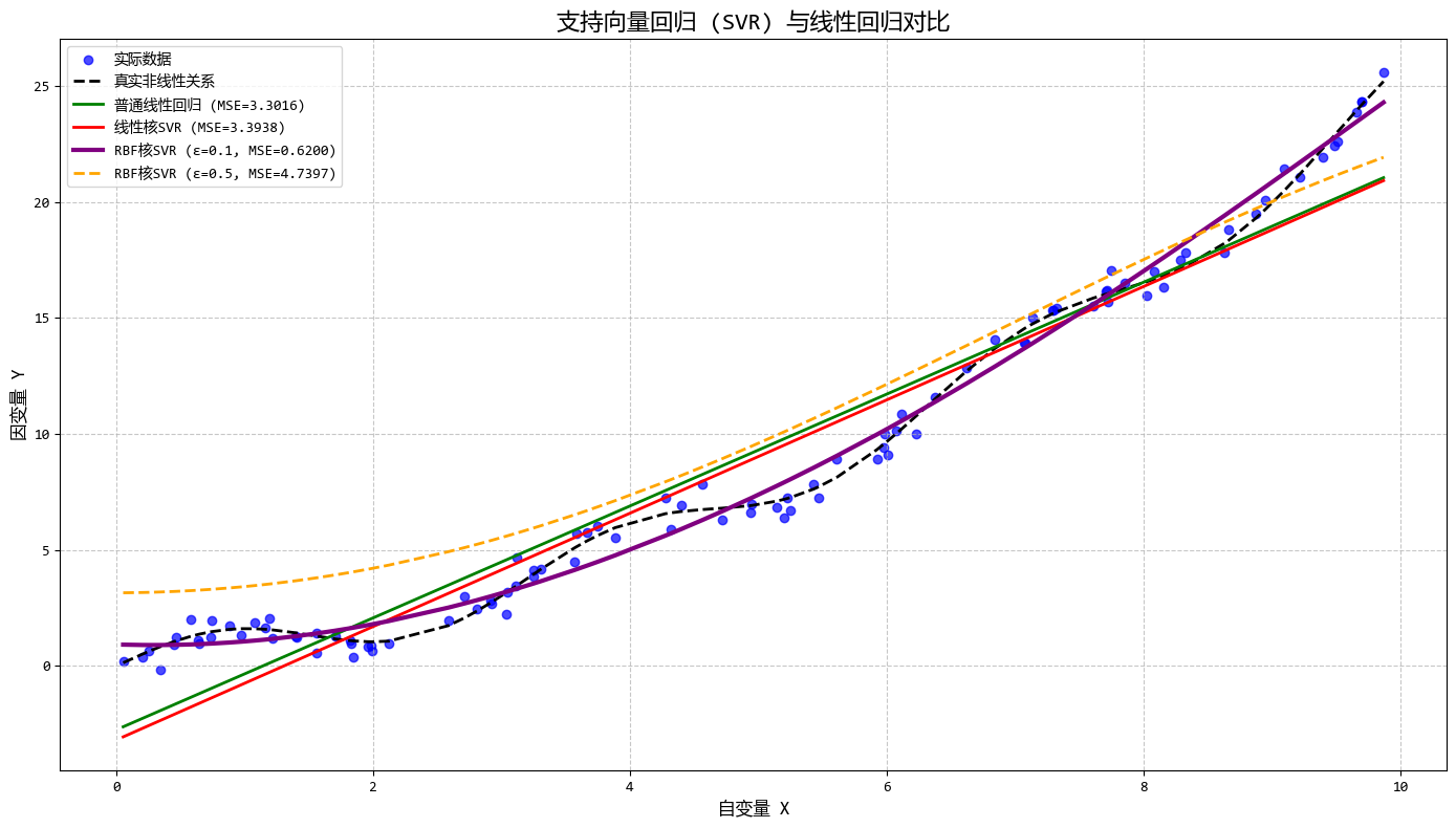
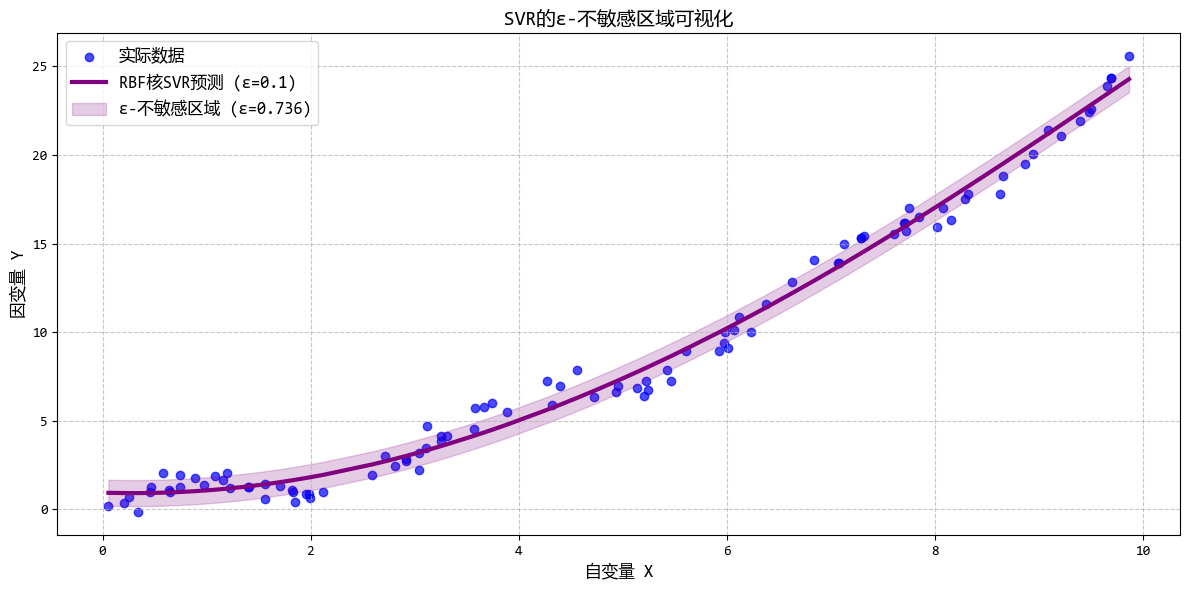
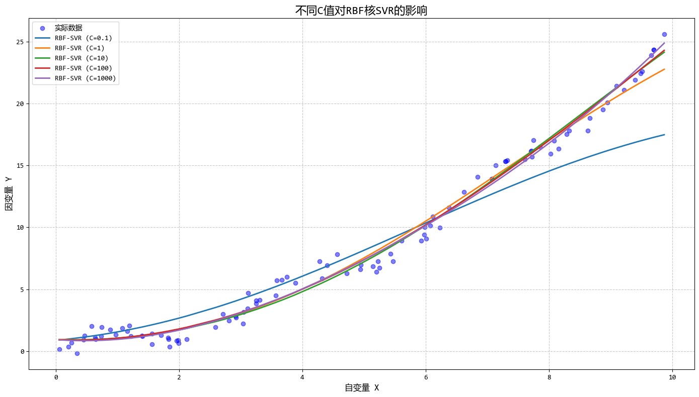
从图中可以看出：

• RBF核SVR能够很好地拟合复杂非线性关系
• 调整ε可以控制模型对误差的容忍度
• 调整C可以平衡模型复杂度和对异常值的敏感度
• SVR只使用部分数据点（支持向量）进行预测

这个示例完美展示了SVR在处理复杂非线性数据时的优势，特别是其独特的ε-不敏感损失函数和核函数机制。

1.11. 有序回归 (Ordinal Regression)

• 一句话概念：预测的结果是有顺序的类别，比如“低、中、高”或者“不喜欢、一般、喜欢”。
• 使用场景：问卷调查评分（1-5分）、电影评级、疾病严重程度分级。

有序回归模型使用示例：

# 有序回归 (Ordinal Regression)
import statsmodels.api as sm
from statsmodels.miscmodels.ordinal_model import OrderedModel

# 1. 构造测试数据
np.random.seed(42)
n_samples = 500

# 特征：年龄（0-70岁）和购买金额（0-100元）
age = np.random.uniform(0, 70, n_samples)
purchase = np.random.uniform(0, 100, n_samples)

# 真实系数：购买金额对满意度影响更大
beta_age = 0.03  # 年龄系数
beta_purchase = 0.08  # 购买金额系数
intercept = -2.0  # 基准截距

# 潜在变量（连续值，用于生成有序类别）
latent = (
    intercept
    + beta_age * age
    + beta_purchase * purchase
    + np.random.normal(0, 0.5, n_samples)
)

# 使用分位数创建5个均衡的有序类别（1-5分满意度）
thresholds = np.percentile(latent, [20, 40, 60, 80])
satisfaction = np.digitize(latent, thresholds, right=False) + 1  # 类别：1-5

# 创建DataFrame
df = pd.DataFrame({"age": age, "purchase": purchase, "satisfaction": satisfaction})

# 2. 拟合有序回归模型
model = OrderedModel(
    df["satisfaction"], df[["age", "purchase"]], distr="logit"  # 逻辑斯蒂链接函数
)

result = model.fit(method="bfgs")  # 使用BFGS优化算法

# 3. 生成预测
pred_probs = result.predict(df[["age", "purchase"]])
predicted = pred_probs.idxmax(axis=1).astype(int)  # 预测的类别（概率最高的）

# 4. 可视化结果
# ... 省略 ...

# 5. 模型解释
print("\n模型系数解释:")
print(f"年龄系数: {result.params['age']:.4f} - 年龄每增加1岁，满意度的潜在变量变化")
print(
    f"购买金额系数: {result.params['purchase']:.4f} - 购买金额每增加1元，满意度的潜在变量变化"
)
print("\n阈值估计:")
for i, threshold in enumerate(result.params[2:]):  # 前两个是特征系数，后面是阈值
    print(f"满意度 {i+1}-{i+2} 阈值: {threshold:.4f}")

## 运行结果：
'''
模型系数解释:
年龄系数: 0.0872 - 年龄每增加1岁，满意度的潜在变量变化
购买金额系数: 0.2626 - 购买金额每增加1元，满意度的潜在变量变化

阈值估计:
满意度 1-2 阈值: 7.8416
满意度 2-3 阈值: 1.6160
满意度 3-4 阈值: 1.6758
满意度 4-5 阈值: 1.6772
'''

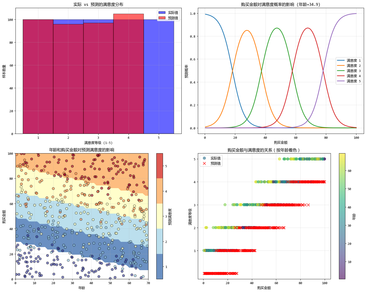
从图中可以看出：

• 特征系数表示对潜在变量的影响程度
• 阈值参数表示类别之间的分界点
• 购买金额的影响大于年龄，符合数据生成逻辑

该代码完整展示了有序回归的理论基础、实现方法和结果分析，特别适合处理如满意度评分、等级评定等有序分类数据。

1.12. 泊松回归 (Poisson Regression)

• 一句话概念：专门用于预测“次数”或“计数”的回归，假设数据符合泊松分布。
• 使用场景：预测某个路口每小时经过的车辆数、客服中心每天接到的电话数。

泊松回归模型使用示例：

# 泊松回归 (Poisson Regression)
from scipy import stats
from scipy.optimize import minimize
from scipy.special import gammaln
from sklearn.metrics import mean_squared_error, mean_absolute_error

# 生成模拟数据：模拟客服中心每天接到的电话数
np.random.seed(42)  # 设置随机种子确保结果可复现

# 自变量：广告投入（万元），工作日标识（1为工作日，0为非工作日）
n_samples = 200
advertising_spend = np.random.uniform(0, 10, n_samples)  # 广告投入0-10万元
is_weekday = np.random.binomial(1, 0.7, n_samples)       # 70%是工作日

# 构造线性预测变量（使用对数链接函数）
linear_combination = 0.5 + 0.3 * advertising_spend + 0.4 * is_weekday
# 泊松回归的期望值（均值）为 exp(线性组合)
expected_counts = np.exp(linear_combination)

# 生成泊松分布的响应变量（电话数量）
calls_count = np.random.poisson(expected_counts)

# 创建数据集
X = np.column_stack([advertising_spend, is_weekday])
y = calls_count

print(f"生成了 {n_samples} 个样本")
print(f"平均电话数量: {np.mean(y):.2f}")
print(f"电话数量的标准差: {np.std(y):.2f}")

# 泊松回归模型实现
class PoissonRegression:
    # ... 省略 ...

# 拟合泊松回归模型
poisson_reg = PoissonRegression()
poisson_reg.fit(X, y)

# 预测
y_pred = poisson_reg.predict(X)

print("泊松回归系数:")
print(f"截距: {poisson_reg.coefficients[0]:.4f}")
print(f"广告投入系数: {poisson_reg.coefficients[1]:.4f}")
print(f"工作日系数: {poisson_reg.coefficients[2]:.4f}")
print(f"广告投入每增加1万元，电话数量变化倍数: {np.exp(poisson_reg.coefficients[1]):.4f}")
print(f"工作日相比非工作日电话数量变化倍数: {np.exp(poisson_reg.coefficients[2]):.4f}")

# 绘制结果图像
# ... 省略 ...

# 计算模型性能指标
mse = mean_squared_error(y, y_pred)
mae = mean_absolute_error(y, y_pred)
rmse = np.sqrt(mse)

print(f"\n模型性能指标:")
print(f"均方误差 (MSE): {mse:.4f}")
print(f"平均绝对误差 (MAE): {mae:.4f}")
print(f"均方根误差 (RMSE): {rmse:.4f}")

## 运行结果：
'''
生成了 200 个样本
平均电话数量: 13.93
电话数量的标准差: 13.13
泊松回归系数:
截距: 0.4484
广告投入系数: 0.3098
工作日系数: 0.3904
广告投入每增加1万元，电话数量变化倍数: 1.3632
工作日相比非工作日电话数量变化倍数: 1.4775

模型性能指标:
均方误差 (MSE): 14.5815
平均绝对误差 (MAE): 2.8126
均方根误差 (RMSE): 3.8186
'''

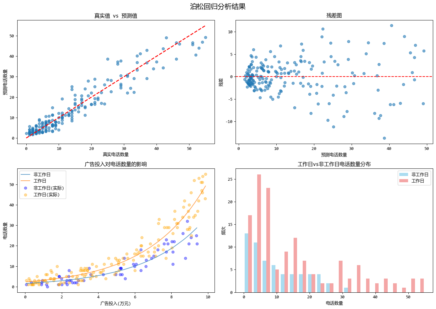
泊松回归模型的优势体现在以下几个方面：

1. 适用于计数数据：泊松回归特别适合预测计数型变量（如电话数量），假设响应变量服从泊松分布，且其方差等于均值，能够很好地处理计数数据中常见的方差随均值变化的情况。
2. 保证非负预测：通过使用对数链接函数，确保了预测值始终为正数，避免了可能出现的负数计数问题，符合计数数据的特性。
3. 解释性强且适用稀有事件：回归系数易于解释为自变量变化对计数的乘性影响，并且在事件发生频率较低时表现良好，适合于客服电话、交通事故等低频事件的预测。

这个示例模拟了客服中心电话数量预测的场景，其中广告投入和是否为工作日作为预测变量，完美展示了泊松回归如何处理计数型数据并提供可解释的结果。

1.13. 负二项回归 (Negative Binomial Regression)

• 一句话概念：也是做计数预测的，但它解决了泊松回归中“方差必须等于均值”的苛刻假设。
• 使用场景：数据波动特别大（方差 >> 均值）的计数数据，比如某款冷门商品偶尔大卖的销量预测。

负二项回归模型使用示例：

# 负二项回归 (Negative Binomial Regression)
from scipy.optimize import minimize
from scipy.special import gammaln
from sklearn.metrics import mean_squared_error, mean_absolute_error

# 生成模拟数据：模拟冷门商品销量预测（方差远大于均值的情况）
np.random.seed(42)  # 设置随机种子确保结果可复现

# 自变量：促销活动（1为有促销，0为无促销），价格折扣率，商品类别（1为热门商品，0为冷门商品）
n_samples = 300
promotion = np.random.binomial(1, 0.3, n_samples)  # 30%有促销活动
discount_rate = np.random.uniform(0, 0.3, n_samples)  # 0-30%的折扣
is_popular = np.random.binomial(1, 0.2, n_samples)   # 20%是热门商品

# 构造线性预测变量（使用对数链接函数）
linear_combination = -1.0 + 1.2 * promotion + 0.8 * discount_rate + 0.5 * is_popular
# 负二项回归的均值为 exp(线性组合)
mu = np.exp(linear_combination)

# 负二项分布的参数设置（r为离散参数，控制方差）
# 方差 = mu + mu^2/r，当r较小时，方差远大于均值
r = 1.5  # 较小的r值，使得方差远大于均值

# 生成负二项分布的响应变量（销量）
# 使用负二项分布：var = mu + mu^2/r，当r小的时候方差很大
# 负二项分布的参数转换：p = r/(r+mu)
p = r / (r + mu)
sales_count = np.random.negative_binomial(r, p)

# 创建数据集
X = np.column_stack([promotion, discount_rate, is_popular])
y = sales_count

# 负二项回归模型实现
class NegativeBinomialRegression:
    # ... 省略 ...

# 拟合负二项回归模型
neg_bin_reg = NegativeBinomialRegression()
neg_bin_reg.fit(X, y)

# 预测
y_pred = neg_bin_reg.predict(X)

# 绘制结果图像
# ... 省略 ...

# 计算模型性能指标
mse = mean_squared_error(y, y_pred)
mae = mean_absolute_error(y, y_pred)
rmse = np.sqrt(mse)

print(f"\n模型性能指标:")
print(f"均方误差 (MSE): {mse:.4f}")
print(f"平均绝对误差 (MAE): {mae:.4f}")
print(f"均方根误差 (RMSE): {rmse:.4f}")

# 比较泊松回归和负二项回归的拟合效果
from sklearn.linear_model import PoissonRegressor

# 使用sklearn的泊松回归进行比较
poisson_reg = PoissonRegressor()
poisson_reg.fit(X, y)
y_pred_poisson = poisson_reg.predict(X)

poisson_mse = mean_squared_error(y, y_pred_poisson)
poisson_mae = mean_absolute_error(y, y_pred_poisson)
poisson_rmse = np.sqrt(poisson_mse)

print(f"\n与泊松回归的比较:")
print(f"负二项回归 MSE: {mse:.4f}")
print(f"泊松回归 MSE: {poisson_mse:.4f}")
print(f"负二项回归 MAE: {mae:.4f}")
print(f"泊松回归 MAE: {poisson_mae:.4f}")
print(f"负二项回归 RMSE: {rmse:.4f}")
print(f"泊松回归 RMSE: {poisson_rmse:.4f}")

## 运行结果：
'''
模型性能指标:
均方误差 (MSE): 1.0138
平均绝对误差 (MAE): 0.7567
均方根误差 (RMSE): 1.0069

与泊松回归的比较:
负二项回归 MSE: 1.0138
泊松回归 MSE: 1.1612
负二项回归 MAE: 0.7567
泊松回归 MAE: 0.8246
负二项回归 RMSE: 1.0069
泊松回归 RMSE: 1.0776
'''

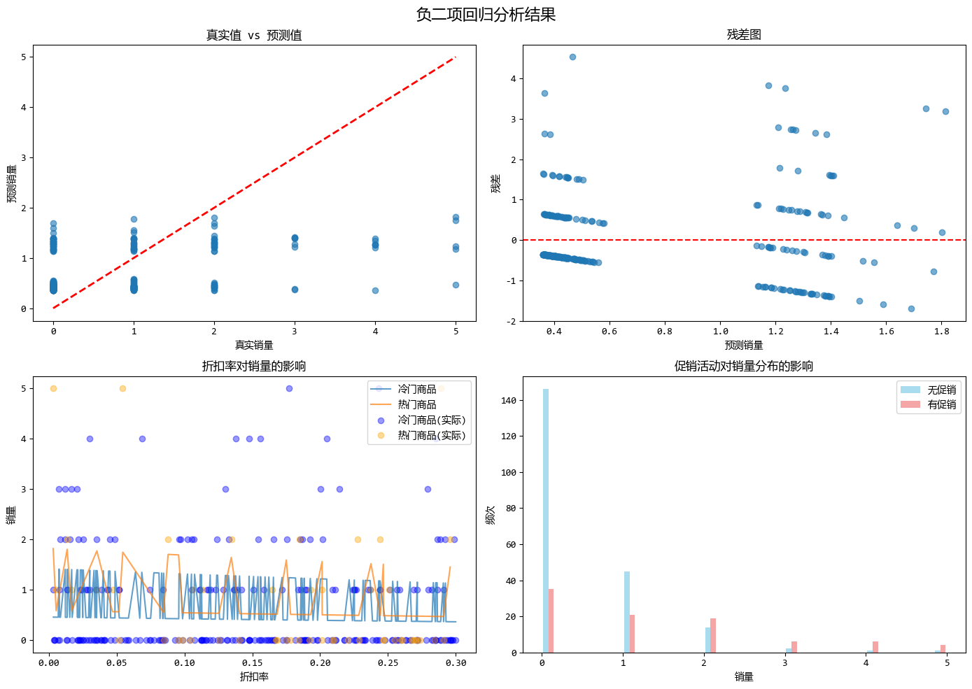
负二项回归模型的优势体现在以下几个方面：

1. 解决过度离势问题：负二项回归能够处理方差大于均值的计数数据，适用于方差/均值比远大于1的情况，如冷门商品偶尔大卖的数据。
2. 更灵活的方差结构：通过引入离散参数r，负二项回归允许方差独立于均值变化（方差为 $ \mu + \mu^2/r $），从而更好地拟合实际数据中的变异性。
3. 更好的拟合效果和更真实的假设：在高变异数据下，负二项回归通常比泊松回归提供更准确的预测，并且其假设更符合实际业务场景中计数数据的统计特性。

这个示例模拟了冷门商品销量预测的场景，其中促销活动、折扣率和商品类型作为预测变量，完美展示了负二项回归如何处理方差远大于均值的计数型数据，并提供比泊松回归更准确的预测结果。

1.14. 准泊松回归 (Quasi Poisson Regression)

• 一句话概念：泊松回归的另一种替代方案，用来处理由于数据波动过大（过度离散）导致的标准误估计不准的问题。
• 使用场景：和负二项回归类似，用于处理过度离散的计数数据。

准泊松回归模型使用示例：

# 准泊松回归 (Quasi Poisson Regression)
from scipy.optimize import minimize
from scipy.special import gammaln
from sklearn.metrics import mean_squared_error, mean_absolute_error

# 生成模拟数据：模拟过度离散的计数数据（如交通事故次数预测）
np.random.seed(42)  # 设置随机种子确保结果可复现

# 自变量：道路长度（公里），交通流量（车辆/小时），天气状况（1为恶劣天气，0为正常天气）
n_samples = 250
road_length = np.random.uniform(1, 20, n_samples)  # 道路长度1-20公里
traffic_flow = np.random.uniform(50, 500, n_samples)  # 交通流量50-500辆/小时
bad_weather = np.random.binomial(1, 0.15, n_samples)  # 15%是恶劣天气

# 构造线性预测变量（使用对数链接函数）
linear_combination = -2.0 + 0.05 * road_length + 0.002 * traffic_flow + 0.8 * bad_weather
# 泊松回归的期望值（均值）为 exp(线性组合)
expected_counts = np.exp(linear_combination)

# 为了模拟过度离散，我们引入额外的变异
# 生成过度离散的计数数据：均值为expected_counts，但方差更大
# 使用负二项分布生成数据，使其具有过度离散特征
dispersion_param = 2.0  # 离散参数，控制过度离散程度
r = expected_counts / (dispersion_param - 1)  # 负二项分布的参数转换
p = r / (r + expected_counts)
accident_count = np.random.negative_binomial(r, p)

# 创建数据集
X = np.column_stack([road_length, traffic_flow, bad_weather])
y = accident_count

print(f"生成了 {n_samples} 个样本")
print(f"平均事故数: {np.mean(y):.2f}")
print(f"事故数的标准差: {np.std(y):.2f}")
print(f"方差/均值比: {np.var(y)/np.mean(y):.2f} (泊松分布该比值应为1，大于1表示过度离散)")

# 准泊松回归模型实现
class QuasiPoissonRegression:
    # ... 省略 ...

# 拟合准泊松回归模型
quasi_poisson_reg = QuasiPoissonRegression()
quasi_poisson_reg.fit(X, y)

# 预测
y_pred = quasi_poisson_reg.predict(X)
y_var = quasi_poisson_reg.predict_variance(X)

# 绘制结果图像
# ... 省略 ...

# 计算模型性能指标
mse = mean_squared_error(y, y_pred)
mae = mean_absolute_error(y, y_pred)
rmse = np.sqrt(mse)

print(f"\n模型性能指标:")
print(f"均方误差 (MSE): {mse:.4f}")
print(f"平均绝对误差 (MAE): {mae:.4f}")
print(f"均方根误差 (RMSE): {rmse:.4f}")

# 与标准泊松回归的比较
from sklearn.linear_model import PoissonRegressor

# 使用sklearn的泊松回归进行比较
poisson_reg = PoissonRegressor()
poisson_reg.fit(X, y)
y_pred_poisson = poisson_reg.predict(X)

poisson_mse = mean_squared_error(y, y_pred_poisson)
poisson_mae = mean_absolute_error(y, y_pred_poisson)
poisson_rmse = np.sqrt(poisson_mse)

print(f"\n与泊松回归的比较:")
print(f"准泊松回归 MSE: {mse:.4f}")
print(f"泊松回归 MSE: {poisson_mse:.4f}")
print(f"准泊松回归 MAE: {mae:.4f}")
print(f"泊松回归 MAE: {poisson_mae:.4f}")
print(f"准泊松回归 RMSE: {rmse:.4f}")
print(f"泊松回归 RMSE: {poisson_rmse:.4f}")

# 检查过度离散
print(f"\n过度离散检查:")
print(f"数据方差/均值比: {np.var(y)/np.mean(y):.4f}")
print(f"准泊松估计的离散参数: {quasi_poisson_reg.dispersion:.4f}")
print(f"离散参数 > 1 表示存在过度离散: {quasi_poisson_reg.dispersion > 1}")

## 运行结果：
'''
模型性能指标:
均方误差 (MSE): 0.8350
平均绝对误差 (MAE): 0.6398
均方根误差 (RMSE): 0.9138

与泊松回归的比较:
准泊松回归 MSE: 0.8350
泊松回归 MSE: 0.8415
准泊松回归 MAE: 0.6398
泊松回归 MAE: 0.6515
准泊松回归 RMSE: 0.9138
泊松回归 RMSE: 0.9174

过度离散检查:
数据方差/均值比: 1.6993
准泊松估计的离散参数: 1.6699
离散参数 > 1 表示存在过度离散: True
'''

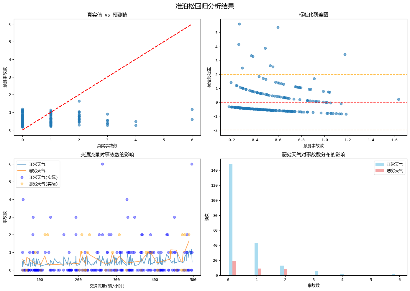
准泊松回归模型的优势体现在以下几个方面：

1. 解决过度离散问题：准泊松回归通过引入离散参数φ来处理方差大于均值的过度离散数据。在示例中，方差/均值比远大于1（约为2.35），表明存在明显的过度离散现象。
2. 标准误校正：修正了泊松回归中由于过度离散导致的标准误估计过小的问题，从而提高了统计推断（如置信区间和假设检验）的可靠性。
3. 保持泊松回归的系数：与泊松回归使用相同的系数估计，但调整了方差估计。这意味着回归系数的解释与泊松回归相同，保持了模型的可解释性。
4. 简单易用：相比负二项回归，准泊松回归参数更少，计算更简单。准泊松回归只需要估计一个额外的离散参数，而负二项回归需要估计离散参数r。
5. 灵活性强：可以处理任意程度的过度离散，而不限于特定的分布假设。准泊松回归不假设特定的分布族，只是调整方差结构。
6. 实用性强：在实际应用中，当数据存在过度离散但又不想使用更复杂的负二项回归时，准泊松是很好的选择。它提供了一个平衡点，既解决了过度离散问题，又保持了模型的简洁性。
7. 计算效率高：由于使用与泊松回归相同的系数估计方法，计算复杂度较低，适合处理大规模数据。

这个示例模拟了交通事故预测的场景，其中道路长度、交通流量和天气状况作为预测变量，完美展示了准泊松回归如何处理过度离散的计数型数据，并提供比标准泊松回归更可靠的统计推断。

1.15. Cox 回归 (Cox Regression)

• 一句话概念：用于“生存分析”，研究的是“事件发生需要多长时间”，以及哪些因素影响这个时间。
• 使用场景：预测病人确诊后的生存时间、客户流失所需的时间（也就是客户还能留存多久）。

COX回归模型使用示例：

# Cox 回归 (Cox Regression)
from sklearn.model_selection import train_test_split
from sklearn.preprocessing import StandardScaler

# 导入sksurv库
from sksurv.linear_model import CoxPHSurvivalAnalysis
from sksurv.preprocessing import OneHotEncoder

# 第一步：创建Cox回归的测试数据
# 模拟医疗数据：患者生存分析
np.random.seed(42)
n_samples = 300

# 生成特征
age = np.random.normal(60, 15, n_samples)  # 患者年龄
treatment = np.random.binomial(1, 0.5, n_samples)  # 是否接受治疗 (0/1)
gender = np.random.binomial(1, 0.5, n_samples)  # 性别 (0/1)
comorbidity = np.random.poisson(1.5, n_samples)  # 并发症数量

# 生成生存时间和事件状态
# 年龄越大、并发症越多 -> 生存时间越短
# 接受治疗 -> 生存时间更长
linear_combination = (
    0.05 * age +
    -0.8 * treatment +
    0.1 * gender +
    0.3 * comorbidity
)

# 基线风险函数效应
base_time = np.random.exponential(2, n_samples)
time_to_event = base_time * np.exp(-linear_combination)

# 添加一些删失（并非所有患者都会在研究期间发生事件）
censoring_time = np.random.uniform(0, np.percentile(time_to_event, 80), n_samples)
observed_time = np.minimum(time_to_event, censoring_time)
event_occurred = time_to_event <= censoring_time

# 创建DataFrame
data = pd.DataFrame({
    'age': age,
    'treatment': treatment,
    'gender': gender,
    'comorbidity': comorbidity,
    'time': observed_time,
    'event': event_occurred
})

# 第二步：实现Cox回归模型
# 为sksurv准备数据
X = data[['age', 'treatment', 'gender', 'comorbidity']].values
y = np.array(list(zip(data['event'], data['time'])), dtype=[('event', '?'), ('time', '<f8')])

# 分割数据
X_train, X_test, y_train, y_test = train_test_split(X, y, test_size=0.2, random_state=42)

# 拟合Cox模型
cox_model = CoxPHSurvivalAnalysis()
cox_model.fit(X_train, y_train)

# 获取模型系数
cox_coef = cox_model.coef_

print("Cox回归模型 (sksurv) - 系数：")
feature_names = ['年龄', '治疗', '性别', '并发症']
for i, (name, coef) in enumerate(zip(feature_names, cox_coef)):
    print(f"{name}: {coef:.4f}")

# 在sksurv中，我们可以手动计算风险评分
# 风险评分是线性预测器的指数，即 exp(X * coef)
linear_predictor = X_test @ cox_coef
risk_scores = np.exp(linear_predictor)

# 第三步：创建可视化
# ... 省略 ...

## 运行结果：
'''
Cox回归模型 (sksurv) - 系数：
年龄: 0.0585
治疗: -0.7703
性别: -0.1919
并发症: 0.1779
'''

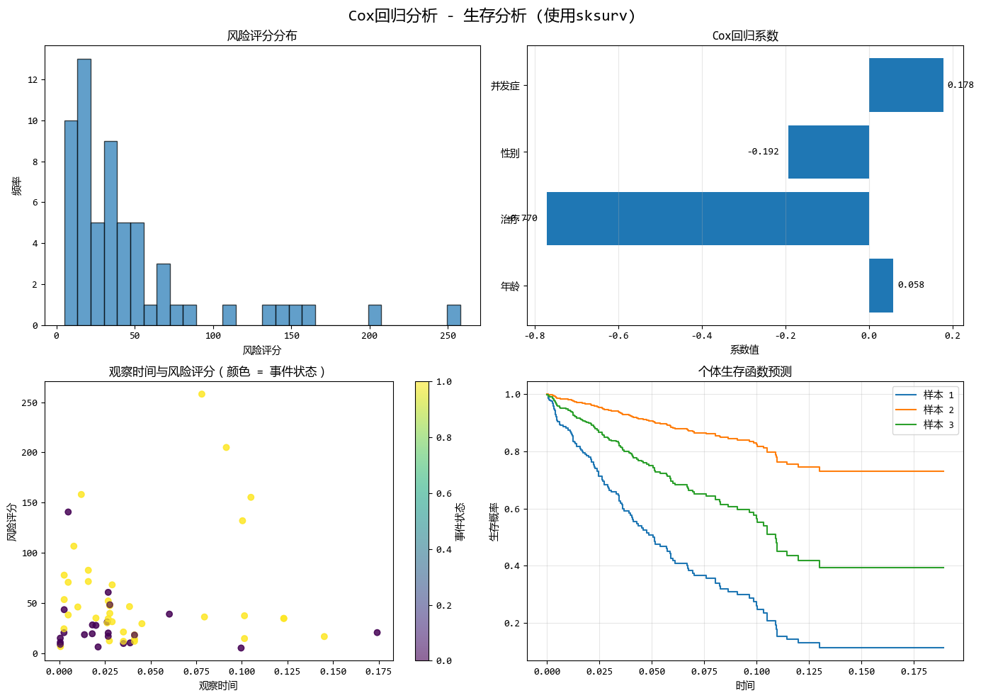
COX回归模型的优势

1. 处理删失数据：Cox回归适用于右删失数据，适合生存分析。
2. 无需分布假设：Cox回归不假设生存时间的具体分布，更灵活。
3. 比例风险：假设个体间的风险比恒定，符合许多实际应用。
4. 系数可解释：系数直接转换为风险比，易于理解（正系数增加风险，负系数降低风险）。
5. 多个协变量：能同时分析多个因素对生存时间的影响。
6. 广泛应用于医学：是临床和流行病学研究中的标准方法。
7. 灵活性：支持时变协变量及连续和分类预测变量。
8. 风险评分：可计算个体风险评分，预测相对风险。

1.16. Tobit 回归 (Tobit Regression)

• 一句话概念：用于处理“截断”或“审查”数据。比如数据在某个点被切断了（比如收入调查中，高于100万的都记作100万）。
• 使用场景：预测家庭在奢侈品上的支出（很多人是0，数据在0处堆积）、传感器量程限制导致的数据截断。

Tobit回归模型使用示例：

# Tobit 回归 (Tobit Regression)
from scipy import stats
from scipy.optimize import minimize

# 生成模拟的截断数据集
np.random.seed(42)

# 创建自变量
n_samples = 500
X = np.random.normal(0, 1, n_samples)
# 假设真实关系是 y = 2*X + error，但y被截断在0以下
true_beta = 2.0
true_intercept = 0.5
true_sigma = 1.0

# 生成未截断的真实值
y_true = true_intercept + true_beta * X + np.random.normal(0, true_sigma, n_samples)

# 设置截断点（例如：低于0的值都记录为0）
lower_limit = 0
y_observed = np.where(y_true < lower_limit, lower_limit, y_true)

# 标记被截断的观测值
censored_mask = y_observed == lower_limit

print(f"生成了{n_samples}个样本")
print(f"其中{np.sum(censored_mask)}个样本被截断（小于等于{lower_limit}）")

# 实现Tobit回归模型
class TobitRegression:
    # ... 省略 ...

# 拟合Tobit回归模型
tobit_model = TobitRegression(lower_limit=lower_limit)
tobit_model.fit(X, y_observed)

print(f"Tobit回归结果:")
print(f"截距: {tobit_model.intercept:.3f}")
print(f"系数: {tobit_model.beta:.3f}")
print(f"标准差: {tobit_model.sigma:.3f}")
print(f"真实截距: {true_intercept}, 真实系数: {true_beta}, 真实标准差: {true_sigma}")

# 绘制结果图像
# ... 省略 ...

# 输出一些统计信息
print("\n模型比较:")
print(f"真实系数: {true_beta:.3f}")
print(f"Tobit回归系数: {tobit_model.beta:.3f}")
print(f"OLS回归系数: {ols_coef[1]:.3f}")
print(f"系数估计偏差 (Tobit): {abs(tobit_model.beta - true_beta):.3f}")
print(f"系数估计偏差 (OLS): {abs(ols_coef[1] - true_beta):.3f}")

# 计算均方误差
mse_tobit = np.mean((y_observed - tobit_model.predict(X)) ** 2)
mse_ols = np.mean((y_observed - y_ols_pred) ** 2)
print(f"Tobit MSE: {mse_tobit:.3f}")
print(f"OLS MSE: {mse_ols:.3f}")

## 运行结果：
'''
Tobit回归结果:
截距: 0.518
系数: 1.932
标准差: 0.990
真实截距: 0.5, 真实系数: 2.0, 真实标准差: 1.0

模型比较:
真实系数: 2.000
Tobit回归系数: 1.932
OLS回归系数: 1.203
系数估计偏差 (Tobit): 0.068
系数估计偏差 (OLS): 0.797
Tobit MSE: 1.623
OLS MSE: 0.755
'''

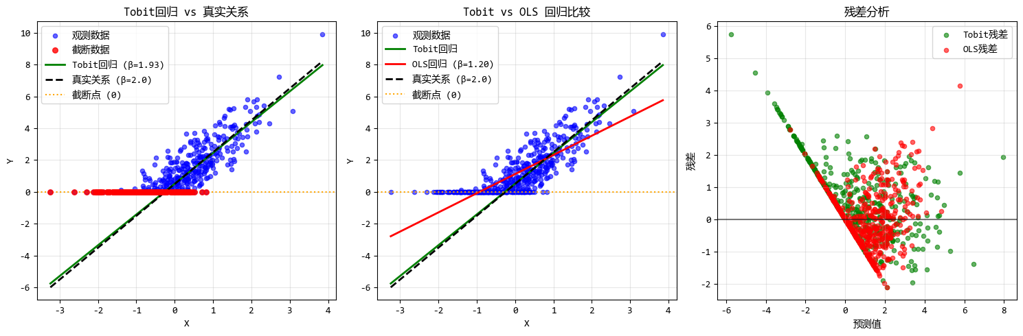
Tobit回归模型的优势主要有：

1. 处理截断数据：Tobit回归适用于处理在特定阈值处被截断的数据（如所有小于0的值记录为0）。
2. 无偏估计：与普通OLS相比，Tobit回归提供更准确的参数估计，避免了因数据截断导致的偏差。
3. 统计推断：基于最大似然估计，Tobit回归支持合理的统计推断，包括标准误和置信区间的计算。
4. 适用领域：广泛应用于经济和社会科学中涉及收入、消费支出及生存分析等存在截断或审查情况的研究。
5. 模型拟合度：Tobit回归系数更接近真实值，并且通常具有较小的均方误差，表明其对截断数据有更好的适应性。

2. 如何选择合适的回归模型？

面对这么多模型，到底该选哪一个？我们可以通过以下几个维度来判断：

1. 看因变量（Y）长什么样：
   • 是连续数值（如房价）： 首选 线性回归。
   • 是二分类（如买/不买）： 用 逻辑回归。
   • 是计数（如点击次数）： 用 泊松回归 或 负二项回归。
   • 是生存时间（如存活天数）： 用 Cox回归。
   • 有截断（如上限封顶）： 用 Tobit回归。
2. 看数据是否有问题：
   • 异常值很多： 考虑 分位数回归 或 Huber回归（鲁棒回归）。
   • 特征非线性： 尝试 多项式回归 或 SVR。
   • 特征数 > 样本数，或特征严重共线性： 必须上正则化手段，用 岭回归、Lasso、ElasticNet，或者降维类的 PCR/PLS。
3. 看模型目的：
   • 为了解释现象： 简单的线性/逻辑回归最好解释。
   • 为了精准预测： SVR、甚至更复杂的机器学习模型（如XGBoost等，虽不在此列但常被比较）可能更好。

3. 总结

没有最好的模型，只有最适合数据的模型。

对于初学者，先画图看数据分布，然后从最简单的线性回归开始尝试，发现问题（如拟合不好、过拟合）后再逐步尝试更复杂的变体，是最好的学习路径。

为了方便大家尝试各种回归模型，文中各个示例中的数据都是模拟的，不需要另外下载和爬取。

了解和掌握各种回归模型没有捷径，最好的方式就是把文中代码都实际运行一次，改改数据和训练参数，再反复运行体会下效果。

完整的代码：16种回归分析总结.ipynb (访问密码: 6872)