bev_feature与真实坐标的关系

1. 推导

在生成 BEV feature 时的 scatter:

nx = int((point_cloud_range[3]-point_cloud_range[0])/voxel_size[0])

# Create the canvas for this sample
canvas = torch.zeros(
    self.in_channels,
    self.nx * self.ny,
    dtype=voxel_features.dtype,
    device=voxel_features.device)

# coors[:,2] 体素y坐标
# coors[:,3] 体素x坐标
indices = coors[:, 2] * self.nx + coors[:, 3]
indices = indices.long()
voxels = voxel_features.t()
# Now scatter the blob back to the canvas.
canvas[:, indices] = voxels
# Undo the column stacking to final 4-dim tensor
canvas = canvas.view(1, self.in_channels, self.ny, self.nx)

示例：

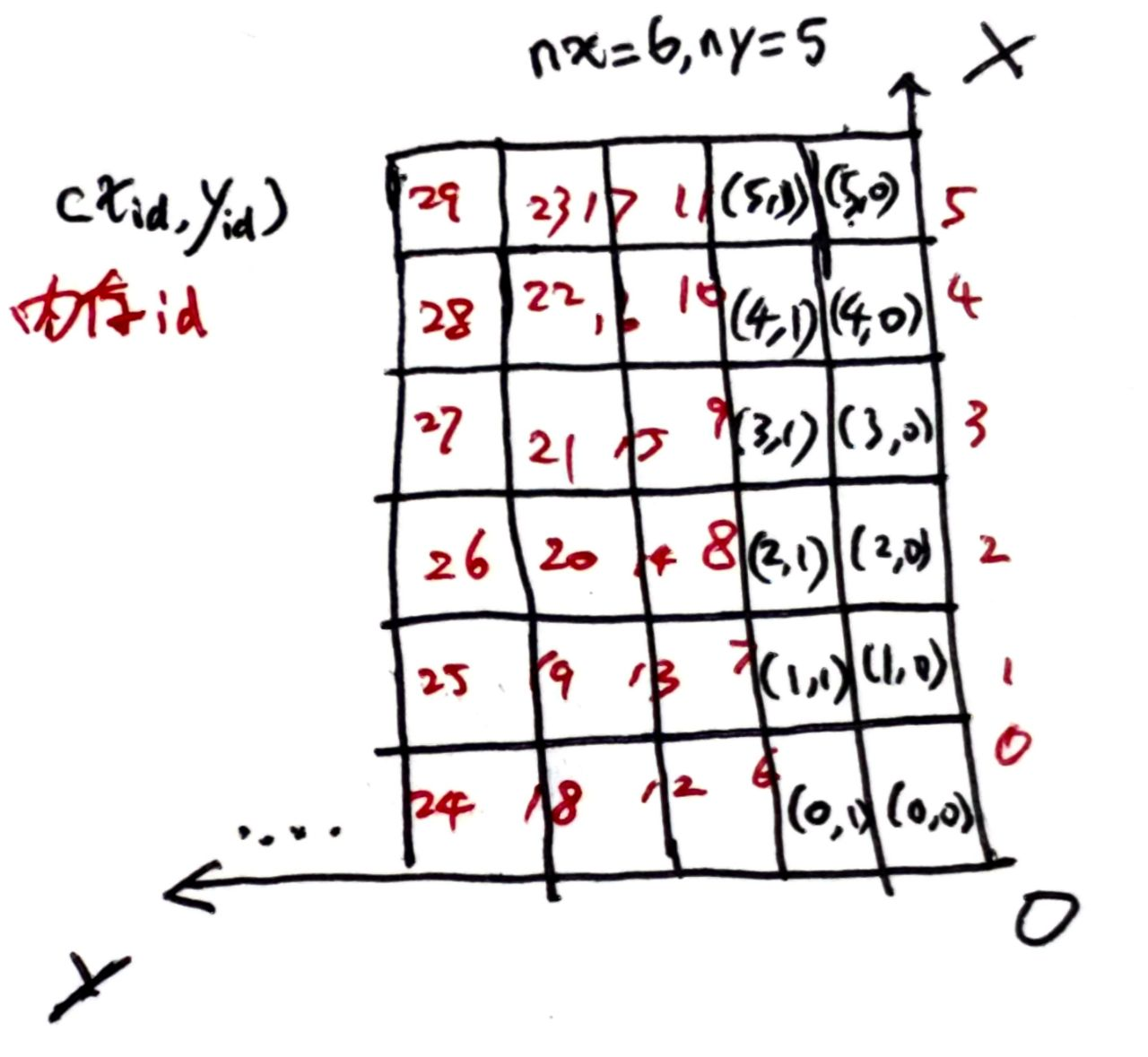
nx = 8
ny = 4
indices = []

for y in range(ny):
    for x in range(nx):
        idx = x + y*nx
        indices.append(idx)

indices_tensor = torch.from_numpy(np.array([indices]))
print(indices_tensor)

indices_tensor = indices_tensor.view(ny, nx)
print(indices_tensor)

indices_tensor = indices_tensor.permute(1, 0)
print(indices_tensor)

result:

tensor([[ 0,  1,  2,  3,  4,  5,  6,  7,  8,  9, 10, 11, 12, 13, 14, 15, 16, 17,
         18, 19, 20, 21, 22, 23, 24, 25, 26, 27, 28, 29, 30, 31]])

tensor([[ 0,  1,  2,  3,  4,  5,  6,  7],
        [ 8,  9, 10, 11, 12, 13, 14, 15],
        [16, 17, 18, 19, 20, 21, 22, 23],
        [24, 25, 26, 27, 28, 29, 30, 31]])

tensor([[ 0,  8, 16, 24],
        [ 1,  9, 17, 25],
        [ 2, 10, 18, 26],
        [ 3, 11, 19, 27],
        [ 4, 12, 20, 28],
        [ 5, 13, 21, 29],
        [ 6, 14, 22, 30],
        [ 7, 15, 23, 31]])

可以看到是按照 x 轴方向，行优先排列的，模型后面所有的操作都是基于这个形状的 feature 做的

occupancy 的输出格式为 1,X,Y,C

# bev_feature: (B, C_i, Dy, Dx)
# (B, C_i, Dy, Dx) -> (B, C_o, Dy, Dx) -> (B, Dx, Dy, C_o)
occ_pred = self.final_conv(bev_feats).permute(0,3,2,1)
bs, Dx, Dy = occ_pred.shape[:3]
# (B, Dx, Dy, C_o) -> (B, Dx, Dy, 2*C_o) ->(B, Dx, Dy, n_cls*Dz)
if self.use_predictor:
    occ_pred = self.predictor(occ_pred)
# (B, Dx, Dy, n_cls*Dz) -> (B, Dx, Dy, Dz, n_cls)
occ_pred = occ_pred.view(bs, Dx, Dy, self.Dz, self.num_classes)

occ_score = occ_pred.softmax(-1)
# (B, Dx, Dy, Dz)
occ_res = occ_score.argmax(-1).float().contiguous()

cuda 得到 point 结果：

int y = coor_idx % occupancy_dim_size.y;
int x = coor_idx / occupancy_dim_size.y;
int occupied_idx = 0;
float lidar_x, lidar_y, lidar_z;
for (int z = 0; z < occupancy_dim_size.z; ++z) {
    int semantic = round(occ_out_deveice[coor_idx * occupancy_dim_size.z + z]);
    if(semantic > 0 && semantic != 2) {
        occupied_idx = atomicAdd(occupied_num_device, 1);
        lidar_x = (x + 0.5) * occupancy_voxel_size.x + range.min_x;
        lidar_y = (y + 0.5) * occupancy_voxel_size.y + range.min_y;
        lidar_z = (z + 0.5) * occupancy_voxel_size.z + range.min_z;

        occupied_out_device[4 * occupied_idx] = lidar_x;
        occupied_out_device[4 * occupied_idx + 1] = lidar_y;
        occupied_out_device[4 * occupied_idx + 2] = lidar_z;
        occupied_out_device[4 * occupied_idx + 3] = semantic;
    }
}

根据 Core Concepts — NVIDIA cuDNN v9.2.1 documentation 的解释

data:

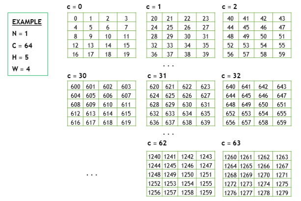
NHWC 排布的数据在内存中的顺序:

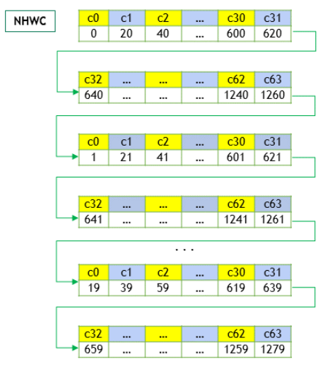
回到 BEV feature map，在 permute(0,3,2,1) 后，2，3 维度是 X, Y 内存是行排列的

int y = coor_idx % occupancy_dim_size.y;
int x = coor_idx / occupancy_dim_size.y;

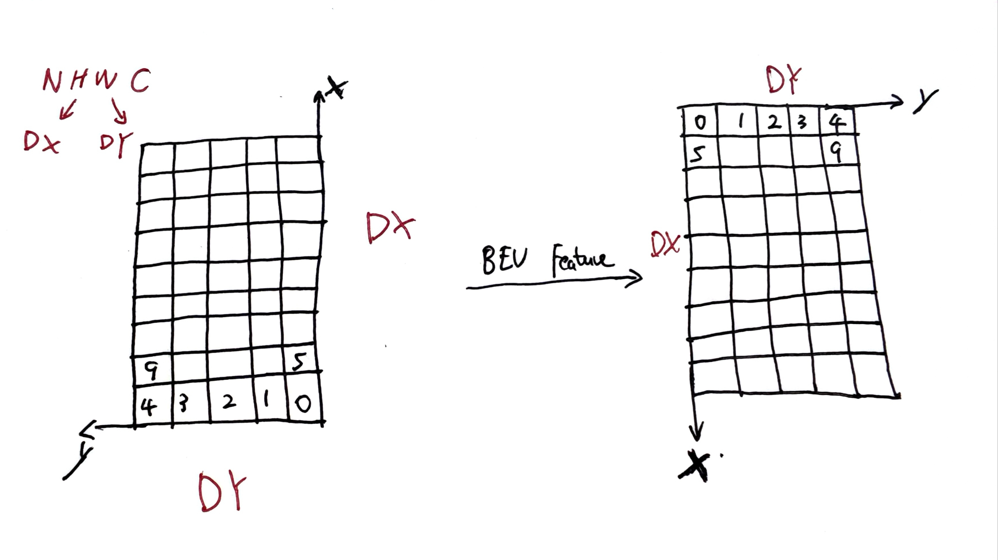
图示：

occ 中的 feature:
这里得到的 BEV feature 与上述一致:

# 真实坐标id
tensor([[ 0,  8, 16, 24], # 第一列在原始BEV中的索引， 映射为内存中的 0,1,2,3
		[ 1,  9, 17, 25],
		[ 2, 10, 18, 26],
		[ 3, 11, 19, 27],
		[ 4, 12, 20, 28],
		[ 5, 13, 21, 29],
		[ 6, 14, 22, 30],
		[ 7, 15, 23, 31]])
# 映射到内存中的id:
tensor([[ 0,  1,  2,  3],
		[ 4,  5,  6,  7],
		[ 8,  9, 10, 11],
		[12, 13, 14, 15],
		[16, 17, 18, 19],
		[20, 21, 22, 23],
		[24, 25, 26, 27],
		[28, 29, 30, 31]])

在目标检测中，centerhead 导出的onnx 最后输出的 feature map 顺序是 1,X,Y,C, 与 occ 是翻转关系：

reg_res = reg_res.permute(0, 2, 3, 1).contiguous()
height_res = height_res.permute(0, 2, 3, 1).contiguous()
dim_res = dim_res.permute(0, 2, 3, 1).contiguous()
rot_res = rot_res.permute(0, 2, 3, 1).contiguous()

数据排布：

tensor([[ 0,  1,  2,  3,  4,  5,  6,  7],
		[ 8,  9, 10, 11, 12, 13, 14, 15],
		[16, 17, 18, 19, 20, 21, 22, 23],
		[24, 25, 26, 27, 28, 29, 30, 31]])

int x = coor_idx % occupancy_dim_size.x;
int y = coor_idx / occupancy_dim_size.x;

2. 实例

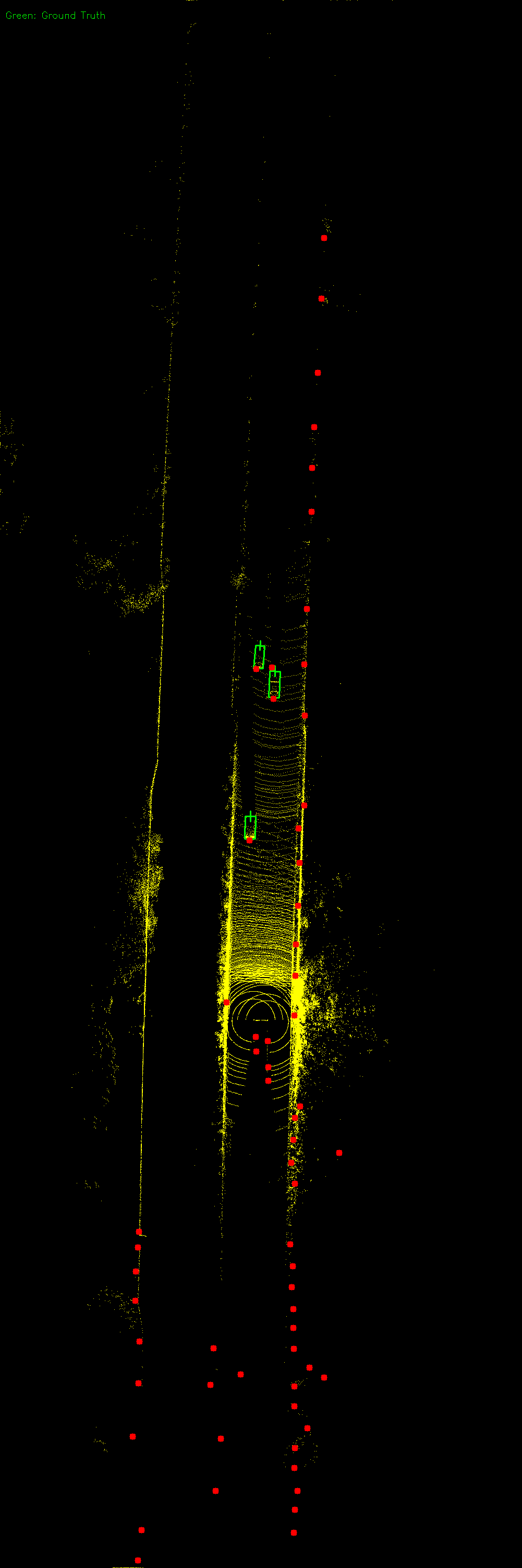
输入点云：

模型参数：
range 范围：
[-50, -51.2, -2, 154.8, 51.2, 6]
voxel 大小：
[0.32, 0.32, 8.0]
原始 BEV 范围：
x: 640, y: 320

pfe 后经过 scatter，输入backbone的 BEV feature map 大小：
[1, 64, 320, 640]
只看尺寸信息，是原始 BEV 的转置，不过是怎样转置的不太清楚，将 feature map 可视化：

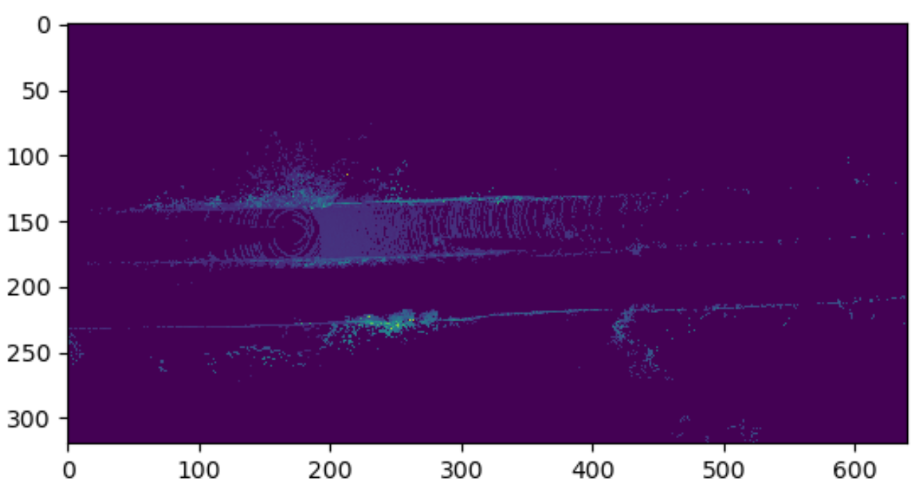
与原始 BEV 图像对比之后，可以看出它们之间的转换关系：

1. 向右旋转 90 度
2. 上下翻转
   lidar 坐标系下一个点 \(p(x,y)\) 到 feature map 坐标 \(u,v\) 或者 \(row,col\) 之间的转换关系：

\[\begin{align} col &= (x-x_{min})/v_x \\ row &= (y-y_{min})/v_y \end{align} \]