Timeseries Prediction Demo base on LSTM

示例代码

import json
import time
import datetime
import requests as req
import numpy as np
import pandas as pd
import matplotlib.pyplot as plt
import matplotlib.dates as mdates
from sklearn.preprocessing import MinMaxScaler
from tensorflow.keras.models import Sequential
from tensorflow.keras.layers import LSTM, Dense
 
 
def date2ts(date_str, layout="%Y-%m-%d %H:%M:%S"):
    date_struct=time.strptime(date_str, layout)
    return int(time.mktime(date_struct))

# 画图之前转换成北京时间
def to_beijing_time(datetime_index):
    return datetime_index.tz_localize('UTC').tz_convert('Asia/Shanghai')
 
# 载入原始数据
with open("dataset_2014.json", "r") as rf:
    c = rf.read()
d = json.loads(c)
data = {}
for i in range(288*3):
    ts = date2ts(d['data']['datetime'][i])
    data[ts] = d['data']['count'][i]
 
 
# 将字典转换为 DataFrame
df = pd.DataFrame(list(data.items()), columns=['timestamp', 'value'])
df['datetime'] = pd.to_datetime(df['timestamp'], unit='s')
df.set_index('datetime', inplace=True)
df.drop('timestamp', axis=1, inplace=True)
 
# 确保数据按时间顺序排序
df = df.sort_index()
 
# 重新采样为 5 分钟间隔，填充缺失值
df = df.resample('5T').mean()
df.interpolate(method='linear', inplace=True)
 
# 数据标准化
scaler = MinMaxScaler(feature_range=(0, 1))
df_scaled = scaler.fit_transform(df)
print("Original Data:\n", df)
print("Scaled Data:\n", df_scaled)
 
# 创建数据集函数
def create_dataset(data, time_step=1):
    X, y = [], []
    for i in range(len(data) - time_step - 1):
        X.append(data[i:(i + time_step), 0])
        y.append(data[i + time_step, 0])
    return np.array(X), np.array(y)
 
 
time_step = 10  # 设定用于输入的时间步长
X, y = create_dataset(df_scaled, time_step)
 
# 拆分训练和测试数据集
train_size = int(len(X) * 0.7)
test_size = len(X) - train_size
X_train, X_test = X[:train_size], X[train_size:]
y_train, y_test = y[:train_size], y[train_size:]
 
# 转换为 LSTM 输入格式
X_train = X_train.reshape(X_train.shape[0], X_train.shape[1], 1)
X_test = X_test.reshape(X_test.shape[0], X_test.shape[1], 1)
 
# 构建 LSTM 模型
model = Sequential()
model.add(LSTM(50, return_sequences=True, input_shape=(time_step, 1)))
model.add(LSTM(50, return_sequences=False))
model.add(Dense(25))
model.add(Dense(1))
 
model.compile(optimizer='adam', loss='mean_squared_error')
model.fit(X_train, y_train, batch_size=1, epochs=10)
 
# 预测
train_predict = model.predict(X_train)
test_predict = model.predict(X_test)
 
# 反标准化预测结果
train_predict = scaler.inverse_transform(train_predict)
test_predict = scaler.inverse_transform(test_predict)
 
# 反标准化实际值
df_inv_scaled = scaler.inverse_transform(df_scaled)
# print("Inverse Scaled Data:\n", df_inv_scaled)
 
# 创建用于绘制图像的空数组
train_predict_plot = np.empty_like(df_scaled)
train_predict_plot[:, :] = np.nan
train_predict_plot[time_step:len(train_predict) + time_step, :] = train_predict
 
# 计算测试预测结果的起始和结束点
start_point = len(train_predict) + time_step  # 设定起始点位置
end_point = start_point + len(test_predict)
test_predict_plot = np.empty_like(df_scaled)
test_predict_plot[:, :] = np.nan
test_predict_plot[start_point:end_point, :] = test_predict[:df_scaled.shape[0] - start_point, :]  # 放置到合适位置
 
# 将时间戳转换回原始时间格式
original = df.index
original_beijing = to_beijing_time(original)
# 创建 figure 绘图
plt.figure(figsize=(15, 6))
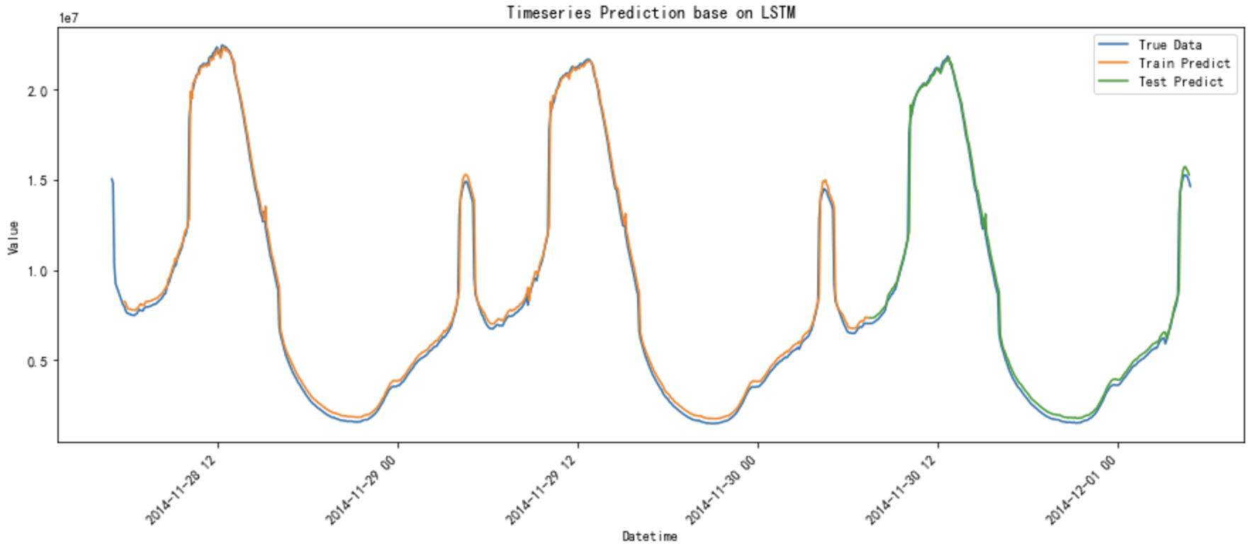
plt.title("Timeseries Prediction base on LSTM")
plt.plot(original_beijing, df_inv_scaled, label='True Data')  # 确保这里使用适当逆标准化数据
plt.plot(original_beijing, train_predict_plot, label='Train Predict')
plt.plot(original_beijing, test_predict_plot, label='Test Predict')
# 格式化 X 轴，提高可读性
plt.gca().xaxis.set_major_locator(mdates.HourLocator(interval=12))
plt.gca().xaxis.set_major_formatter(mdates.DateFormatter('%Y-%m-%d %H:%M', tz=original_beijing.tz))
plt.gcf().autofmt_xdate(rotation=45)
plt.xlabel('Datetime')
plt.ylabel('Value')
plt.legend()
plt.show()


# # 提取最后3天的数据
# last_three_days_mask = original >= (original.max() - pd.Timedelta(days=3))
# filtered_original = original[last_three_days_mask]
# filtered_df_inv_scaled = df_inv_scaled[last_three_days_mask]
# filtered_train_predict_plot = train_predict_plot[last_three_days_mask]
# filtered_test_predict_plot = test_predict_plot[last_three_days_mask]
# # 转换时间为北京时间
# filtered_original_beijing = to_beijing_time(filtered_original)

# plt.figure(figsize=(15, 6))
# plt.title("Timeseries Prediction base on LSTM （last 3 days）")
# plt.plot(filtered_original_beijing, filtered_df_inv_scaled, label='True Data')  # 确保这里使用适当逆标准化数据
# plt.plot(filtered_original_beijing, filtered_train_predict_plot, label='Train Predict')
# plt.plot(filtered_original_beijing, filtered_test_predict_plot, label='Test Predict')
# # 格式化 X 轴使用年，并倾斜显示
# plt.gca().xaxis.set_major_locator(mdates.HourLocator(interval=4))
# plt.gca().xaxis.set_major_formatter(mdates.DateFormatter('%Y-%m-%d %H:%M', tz=filtered_original_beijing.tz))
# plt.gcf().autofmt_xdate(rotation=45)
# plt.xlabel('Datetime')
# plt.ylabel('Value')
# plt.legend()
# plt.show()

效果对比