Pointnet+Frustum-Pointnet复现(Pytorch1.3+Ubuntu18.04)
2020.05.08
这篇博文是好久以前复现代码的时候顺手写的,但当时没时间手写pointnet++了,只写了frstum_pointnets_pytorch(https://github.com/simon3dv/frustum_pointnets_pytorch),再后来的实验又改了PointRCNN作为baseline, 所以这边就一直没更新下去了, 而且后面的东西写得很乱, 导致这篇博文屯了几个月都还没发布, 现在想了想还是发布了吧.
本文是对复现代码的解释,完整代码在simon3dv/PointNet1_2_pytorch_reproduced (ps:当时只写完pointnet就没时间更下去了, 反正现在pointnet++已经有至少两个pytorch版本了, 所以我也没更)
1.数据集和预处理
/experiments/prepare_data.ipynb
1.1 ModelNet40
ModelNet40是一个大规模3D CAD数据集,始于3D ShapeNets: A Deep Representation for Volumetric Shapes
Zhirong,创建初衷是为了学习到能良好捕捉类内差别的3D表示,比当时最新的数据集大22倍。包含151,128个3D CAD模型和660个不同类别,如下图。

作者在实验时仅选取了40个类别,每个类别各100个不同的CAD模型,得到4000个CAD模型。(但我下载出来的ModelNet40并不是4000个CAD模型,而是训练集有9843个,测试集有2468个,而且类内数量不同)
1.1.1 ModelNet10
ModelNet10选取了对应于NYU RGB-D数据集的其中10个类别。
1.1.2 原始数据分析和可视化
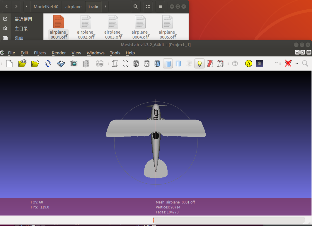
这里CAD模型是.off格式,可以在ubuntu上用meshlab进行可视化,可以旋转缩放。
比如airplane_0001.off
OFF
90714 104773 0
20.967 -26.1154 46.5444
21.0619 -26.091 46.5031
-1.08889 46.8341 38.0388
3 24 25 26  <--第90717行
3 25 24 27
...
3 90711 90710 90713  <--第195489行
第二行三个参数表示有90714个顶点,104773个面,0个边。
然后是90714行,每行是点的坐标。
最后是104773行,每行表示面,3指3个点,24 25 26指点的索引。
在meshlab中可以看到:
Pointet官方提供的数据是已经处理过的.h5格式,而非ModelNet40的.OFF,而且并没有给出读取OFF并写入.h5的代码,却有读取ply的代码。

以其中一个ply_data_train0.h5为例,查看其中的数据
import numpy as np
import h5py
import os
#example of a single ply_data_train0.h5
f = h5py.File('modelnet40_ply_hdf5_2048/ply_data_train0.h5', 'r')
dset = f.keys()#<KeysViewHDF5 ['data', 'faceId', 'label', 'normal']>
data = f['data'][:]#(2048, 2048, 3),dtype=float32,min=-0.9999981,max=0.9999962,mean=2.1612625e-09
faceId = f['faceId'][:]#(2048, 2048),dtype=int32,min=0,max=1435033
label = f['label'][:]#(2048,1),dtype=uint8,min=0,max=39
normal = f['normal'][:]#(2048, 2048, 3),dtype=float32,min=-1.0,max=1.0,mean=-0.0041686897
对于此,PointNet论文中已经有所解释,
We uniformly sample 1024 points on mesh faces according to face area and normalize them into a unit sphere.During training we augment the point cloud on-the-fly by randomly rotating the object along the up-axis and jitter the position of each points by a Gaussian noise with zero mean and 0.02 standard deviation.(在网格面上均匀采样1024个点,标准化为单位圆。训练时增强数据:一是沿up-axis随机旋转,二是点云抖动,对每个点增加一个噪声位移,噪声的均值为0,标准差为0.02)
可以推理出,data是从均匀采样后且标准化为单位圆后的2048个点,faceId是2048个点对应的面的序号,label是类别标签,normal是法向量。为了验证data是否已标准化,我做了以下验证,求点云的直径,标准化后应该为1。可以看出已经很接近1了(但不清楚为什么有点误差)。
>>> np.max(np.sqrt(np.sum(abs(data[1])**2,axis=-1)))
0.94388014
>>> np.max(np.sqrt(np.sum(abs(data[2])**2,axis=-1)))
0.9544609
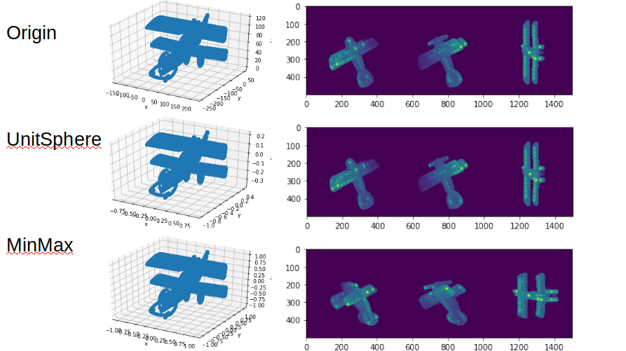
可以看出normal确实是对data标准化为单位圆后的结果。这里对标准化的方法进一步分析, pointnet/utils/pc_util.py 中有以下代码,可以直接使用。这里标准化是用点云/直径的方式,如果用min-max标准化会导致变形。
    # Normalize the point cloud
    # We normalize scale to fit points in a unit sphere
    if normalize:
        centroid = np.mean(points, axis=0)
        points -= centroid
        furthest_distance = np.max(np.sqrt(np.sum(abs(points)**2,axis=-1)))
        points /= furthest_distance
利用pointnet/utils/pc_util.py中的可视化函数,plot出标准化后的点云如下,完整代码在simon3dv/PointNet1_2_pytorch_reproduced/experiments/prepare_data.ipynb
。
接下来回来继续看Pointnet官方,整个文件夹一共有7个.h5文件,应该包括了整个训练集和测试集。
# all .h5
datapath = 'modelnet40_ply_hdf5_2048'
for root, dirs, files in os.walk(datapath):
    for _f in files:
        if(_f.endswith('.h5')):
            f = h5py.File(os.path.join(datapath,_f), 'r')
            dset = f.keys()
            data = f['data'][:]
            print(_f,data.shape)
'''Results
ply_data_train1.h5 (2048, 2048, 3)
ply_data_test0.h5 (2048, 2048, 3)
ply_data_train2.h5 (2048, 2048, 3)
ply_data_test1.h5 (420, 2048, 3)
ply_data_train3.h5 (2048, 2048, 3)
ply_data_train4.h5 (1648, 2048, 3)
ply_data_train0.h5 (2048, 2048, 3)
可以看到,train有5个.h5,一共是9840个(2048,3)维的点,而test有2个.h5,一共有2468个点,与论文里说的一致。
1.1.3 随机采样
“在网格面上均匀采样1024个点,标准化为单位圆。”我的代码如下(由于pointnet没给采样代码,这里先用最简单的随机采样进行实现):
npoints = 1024
points = points_unit_sphere
choice = np.random.choice(len(faces), npoints, replace=True)
idxs = faces[choice,1:]
points_subset = np.mean(points[idxs],axis=1)
pyplot_draw_point_cloud(points_subset,'points_subset')
运行结果:

也可以直接从N个顶点中选1024个,有的人是这么实现的,不知道会不会影响结果:
points = points_unit_sphere
choice = np.random.choice(len(points), npoints, replace=True)
points_subset = points[choice, :]
pyplot_draw_point_cloud(points_subset,'points_subset')
运行结果:

1.1.4 最远点采样
后来发现随机采样效果很差,于是做了以下最远点采样的可视化。(最远点采样也是均匀采样的一种)

最远点采样的思想很简单,即一个一个选点,要求当前点的选取与上一个点的距离最大;但速度也比较慢,从151185个点采样到1024要花Time 3.887915030005388s,相比随机采样的Time 0.001566361985169351 s增大了1000倍。代码如下,参考了博客https://blog.csdn.net/weixin_39373480/article/details/88878629#37__330
def farthest_point_sample(xyz, npoint):
    N, C = xyz.shape
    centroids = np.zeros(npoint)
    distance = np.ones(N) * 1e10
    farthest = np.random.randint(0, N)# random select one as centroid
    for i in range(npoint):
        centroids[i] = farthest
        centroid = xyz[farthest, :].reshape(1, 3)
        dist = np.sum((xyz - centroid) ** 2, -1)
        mask = dist < distance
        distance[mask] = dist[mask]
        farthest = np.argmax(distance)# select the farthest one as centroid
        #print('index:%d, dis:%.3f'%(farthest,np.max(distance)))
    return centroids
xyz = points.copy()
start = time.perf_counter()
points_farthest_index = farthest_point_sample(xyz,1024).astype(np.int64)
points_farthest = xyz[points_farthest_index,:]
print("%d to %d"%(xyz.shape[0],points_farthest.shape[0]))
print("Time {} s".format(float(time.perf_counter()-start)))
1.1.5 数据增强
Pointnet论文中训练时增强数据:一是沿垂直方向随机旋转,二是点云抖动,对每个点增加一个噪声位移,噪声的均值为0,标准差为0.02,我的代码如下:
    def data_aug(self, points):
        if self.rotation:
            theta = np.random.uniform(0, np.pi * 2)
            rotation_matrix = np.array([[np.cos(theta), -np.sin(theta)], [np.sin(theta), np.cos(theta)]])
            points[:, [0, 2]] = points[:, [0, 2]].dot(rotation_matrix)  # random rotation
        if self.jiggle:
            points += np.clip(np.random.normal(0, 0.01, size=points.shape),-0.05,0.05)  # random jitter
        return points
运行结果

1.2 ShapeNet
ShapeNet也是一个大型3D CAD数据集,包含3Million+ models and 4K+ categories。旨在采用一种数据驱动的方法来从各个对象类别和姿势的原始3D数据中学习复杂的形状分布(比如看到杯子侧面就能预测到里面是空心的),并自动发现分层的组合式零件表示。包含的任务有:object category recognition, shape completion, part segmentation,Next-Best-View Prediction, 3D Mesh Retrieval.但是,ShapeNet(这篇文章中)使用的模型采用卷积深度置信网络将几何3D形状表示为3D体素网格上二进制变量的概率分布,而不是像后来出现的PointNet那样直接以点云的原始形式作为输入。
1.2.1 ShapeNet
PointNet用的是其中的子集,包含16881个形状,16个类别,50个部件,标签在采样点上。下载连接在shapenetcore_partanno_v0(pre-released)(1.08GB),shapenetcore_partanno_segmentation_benchmark_v0()(635MB) 或者 pointnet作者提供的shapenet_part_seg_hdf5_data(346MB)
1.2.2 原始数据分析和可视化
为了方便起见,这里直接用pointnet作者提供的shapenet_part_seg_hdf5_data(346MB)。

test_file = '/home/aming/文档/reproduced/PointNet1_2_pytorch_reproduced/data/ShapeNet/hdf5_data/ply_data_test0.h5'
f = h5py.File(test_file, 'r')
dset = f.keys()#<KeysViewHDF5 ['data', 'label', 'pid']>
data = f['data']#(2048, 2048, 3)
label = f['label']#(2048, 1)
pid = f['pid']#(2048, 2048)
points = data[0]
pyplot_draw_point_cloud(points,'points1')

接下来对分割进行着色:
2 我的pytorch版复现
2.1 Dataset创建
2.1.1 .h5 or .off ?
首先遇到的一个问题是,PointNet提供了预处理好的9840个训练数据和2468个测试数据,包括单位球标准化和采样2048个点,但不包括数据增强(随机旋转和抖动)。在modelnet40_ply_hdf5_2048文件夹中以多个.h5文件存储。然而,ModelNet官方提供的ModelNet40则是.off格式。
我首先尝试在Dataset的__getitem__中从.off中读取所有点和面,但发现这导致了GPU利用率为0,因为读取太慢(点数面数很多的时候,一个.off要读0.72s)。
然后,为了提高gpu利用率,我先用
train_points, train_label, test_points, test_label = \
            load_data(root_dir=args.datapath,setting_dir=args.settingpath)
将所有数据导入,在Dataset创建时传入所有数据。但仍然有一个问题:每次训练开始都要读二十分钟的数据,很不方便调试。最后,我对所有数据先单位球标准化,再随机从网格面采样2048个点,然后保存为.h5格式。
def export_h5_from_off(root_dir,out_dir):
    cat = []
    for x in os.listdir(root_dir):
        if (len(x.split('.')) == 1):
            cat.append(x)
    from dataset_util import save_h5,read_off,samplen,unit_sphere_norm
    for split in ['train','test']:
        h5_dir = os.path.join(out_dir,split)
        if not os.path.exists(h5_dir):
            os.makedirs(h5_dir)
        for i in range(len(cat)):
            filenames = os.listdir(os.path.join(root_dir, cat[i],split))
            all_points = np.zeros((len(filenames),2048,3))
            for j,x in enumerate(filenames):
                filename = os.path.join(root_dir, cat[i], split, x)
                out = os.path.join(root_dir, cat[i], split, x)
                points, faces = read_off(filename)
                points = unit_sphere_norm(points)
                points = samplen(points,faces)
                all_points[j,:,:] = points
            label = np.zeros((len(filenames),1))
            label[:] = i
            outname = cat[i]+'.h5'
            save_h5(os.path.join(out_dir, split, outname), all_points, label)
            print('writing %s (%d %s) done'%(cat[i],len(filenames),split))
def load_h5(h5_filename):
    f = h5py.File(h5_filename)
    data = f['data'][:]
    label = f['label'][:]
    seg = []
    return (data, label, seg)

def load_data_from_h5(root_dir,classification=True):
    split = 'train'
    train_data_list = []
    train_label_list = []
    train_dir = os.path.join(root_dir, split)
    filenames = os.listdir(train_dir)
    for i,filename in enumerate(filenames):
        data,label,seg = load_h5(os.path.join(train_dir,filename))
        train_data_list.append(data)
        train_label_list.append(label)
    train_data = np.concatenate(train_data_list)
    train_label = np.concatenate(train_label_list)
    print('train_data:',train_data.shape)
    print('train_label:',train_label.shape)

    split = 'test'
    test_data_list = []
    test_label_list = []
    test_dir = os.path.join(root_dir, split)
    filenames = os.listdir(test_dir)
    for i,filename in enumerate(filenames):
        data,label,seg = load_h5(os.path.join(test_dir,filename))
        test_data_list.append(data)
        test_label_list.append(label)
    test_data = np.concatenate(test_data_list)
    test_label = np.concatenate(test_label_list)
    print('train_data:',test_data.shape)
    print('train_label:',test_label.shape)

    if classification:
        return train_data, train_label, test_data, test_label
2.1.2 数据集预处理问题(已解决)
见3.1.6 ModelNet40 mesh_sample,预处理用mesh_sample(random即可)的方法,要考虑面积加权,最后准确率才会比较高。直接用点采样的话哪怕用fps准确率也会下降0.03.
2.2 训练
2.2.1 T-Net的训练(初始化、损失函数)
PointNet官方代码对T-Net的fc3对weight零初始化,bias初始化为单位矩阵。我在实验中也发现,如果不这么做,准确率在第一个epoch就非常低,后面很难超越不加T-Net的方案。tensorflow代码为
    with tf.variable_scope('transform_XYZ') as sc:
        assert(K==3)
        weights = tf.get_variable('weights', [256, 3*K],
                                  initializer=tf.constant_initializer(0.0),
                                  dtype=tf.float32)
        biases = tf.get_variable('biases', [3*K],
                                 initializer=tf.constant_initializer(0.0),
                                 dtype=tf.float32)
        biases += tf.constant([1,0,0,0,1,0,0,0,1], dtype=tf.float32)
        transform = tf.matmul(net, weights)
        transform = tf.nn.bias_add(transform, biases)
我的代码为
    self.fc3 = nn.Linear(256,9)
    init.zeors_(self.fc3.weight)#init.constant_(self.fc3.weight,1e-8)
    self.fc3.bias.data = torch.eye(3, requires_grad=True).flatten()
对于损失函数,官方是在softmax classification loss基础上加一个0.001权重的L2范数,代码如下。
def get_loss(pred, label, end_points, reg_weight=0.001):
    """ pred: B*NUM_CLASSES,
        label: B, """
    loss = tf.nn.sparse_softmax_cross_entropy_with_logits(logits=pred, labels=label)
    classify_loss = tf.reduce_mean(loss)
    tf.summary.scalar('classify loss', classify_loss)

    # Enforce the transformation as orthogonal matrix
    transform = end_points['transform'] # BxKxK
    K = transform.get_shape()[1].value
    mat_diff = tf.matmul(transform, tf.transpose(transform, perm=[0,2,1]))
    mat_diff -= tf.constant(np.eye(K), dtype=tf.float32)
    mat_diff_loss = tf.nn.l2_loss(mat_diff)
    tf.summary.scalar('mat loss', mat_diff_loss)

    return classify_loss + mat_diff_loss * reg_weight
首先,tf.nn.l2_loss返回的是output = sum(t ** 2) / 2,所以其实不是l2_loss,既没有开方,还除以了2.
在pytorch中,可以用torch.norm(X-I)实现,也可以用torch.nn.functional.mse_loss(X,I,reduction='sum')实现。但torch.norm默认开根号【而且我用torch.norm()配合零初始化后在第二个batch参数会全变成nan,改成torch.norm()+1e-8就没问题,或者改成mse_loss+0初始化也没问题,不知为何】
其次,不知道为什么官方的tf.nn.l2_loss(mat_diff) 没有除以batchsize,我实现时除了,对0.001的权重也做了相应调整。
2.2.2 分类损失函数(不含stn)
对于分类,包含softmax classification loss和T-Net的regularization loss (with weight 0.001)。
官方tensorflow代码为
    loss = tf.nn.sparse_softmax_cross_entropy_with_logits(logits=pred, labels=label)
    classify_loss = tf.reduce_mean(loss)#相当于除以batch_size
这个tf.nn.sparse_softmax_cross_entropy_with_logits要注意两部分:
1.其功能是做一次softmax再算交叉熵:
2.输入的labels是index,而非one-hot
其数学表达式为
(其中\(y_{i}^{\prime}\)是标签,\(y_i\)是预测值)
在pytorch复现时,常用用两个函数搭配来实现:
    #pointnet.py中
    ...
    x = self.fc3(x)
    return F.log_softmax(x,dim=1), ...
    #trainCls.py中
    loss = F.nll_loss(pred,target)#compute x[class]
其中F.nll_loss是negative log likelihood loss,但输入的是一个对数概率向量和一个标签,不会为我们计算对数,所以最好配合F.log_softmax使用。
2.2.3 关键点集和上界点集可视化
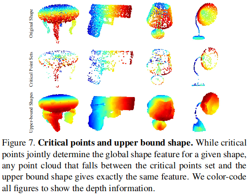
从(bs,n_points,1024)的逐点特征maxpool成(bs,1,1024)的全局特征时,这n_points个点对全局特征的贡献不同。有的点去掉不会影响全局特征,因为这个点的1024维特征在maxpool时都没有取到最大值;而另一些点去掉就会改变全局特征,这些点称为“关键点”,是原始点云的子集。而上界点集,可以理解为从[-1,1] x [-1,1] x -1,1遍历所有的点,如果一个点加入原始点云中不改变全局特征,则这个点在上界点集中,因此,原始点云是上界点集的子集。
pointnet的官方github并没有发布求关键点集和上界点集的方法,为此我自己做了简单的实现:
对于关键点集,只要在pointnet做maxpool时返回索引即可
index = torch.max(x, 2)[1]
而对于上界点集,则首先在原始点云中找到一个非关键点的点,(这是为了方便加入新的一个点)
    choice = 0
    while choice in index_cs: #select a non-critical point
        choice += 1
然后遍历标准化后的空间的所有点,并替换刚刚找到的非关键点的点,然后求全局特征,如果全局特征发生改变,则加入上界点集。
    for x in np.arange(-1,1,search_step):
        for y in np.arange(-1,1,search_step):
            for z in np.arange(-1,1,search_step):
                xyz = torch.tensor([x,y,z],dtype=torch.float32)
                points[0,:,choice] = xyz
                global_feat, _ = classifier(points)
                if (global_feat.detach() <= global_feat_original.detach()).all():
                    ub = np.append(ub, np.array([[x,y,z]]),axis = 0)
我的结果如下:

更详细的资料可以参考WindWing的工作,里面有代码和一个详细的report。
3.训练结果和一些小实验
3.1 ModelNet40
3.1.1 简单版本
对于ModelNet40的分类,采用默认参数:(epoch=135(BestEpoch), batchsize=16, Adam(learning_rate=0.001,weight_decay=1e-4),no data_augumentation,no T-Net)
python trainCls.py --name Default
Your args:
Namespace(bs=16, datapath='./data/modelnet40_ply_hdf5_2048', dr=0.0001, gamma=0.7, jiggle=False, ks=1, lr=0.001, mode='train', model=None, name='Default', nepochs=300, optimizer='Adam', outf='./output/pointnet', rotation=False, seed=1, stn1=False, stn2=False, stn3=False, stn4=False, test_npoints=2048, train_npoints=2048, weight3=0.0005, weight64=0.0005, workers=4)
...
[300: 614/615] test loss: 0.026663 accuracy: 0.885081
Best Test Accuracy: 0.893145(Epoch 261)
100%|█████████████████████████████████████████████| 155/155 [00:00<00:00, 158.63it/s]
final accuracy 0.8850806451612904
Time 59.86838314503354 min
3.1.2 +T-Net
#3x3 only
CUDA_VISIBLE_DEVICES=0 python trainCls.py --name Default_stn1 --stn1
Best Test Accuracy: 0.897984(Epoch 124)
100%|██████████████████████████████████████████████| 155/155 [00:01<00:00, 91.87it/s]
final accuracy 0.8879032258064516
Time 109.93467423691666 min
#64x64 only
CUDA_VISIBLE_DEVICES=1 python trainCls.py --name Default_stn2 --stn2
Best Test Accuracy: 0.894355(Epoch 177)
100%|█████████████████████████████████████████| 155/155 [00:01<00:00, 88.42it/s]
final accuracy 0.8858870967741935
Time 114.30135896029994 min
#论文提到的3x3 + 64x64 + reg64
CUDA_VISIBLE_DEVICES=0 python trainCls.py --name Default_stn123 --
stn1 --stn2 --stn3
[300: 614/615] test loss: 0.026368 accuracy: 0.892339
Best Test Accuracy: 0.899597(Epoch 188)
100%|█████████████████████████████████████████| 155/155 [00:02<00:00, 62.45it/s]
final accuracy 0.8923387096774194
Time 170.0766429228 min
#try 3x3 + reg3
CUDA_VISIBLE_DEVICES=0 python trainCls.py --name Default_stn14 --stn1 --stn4
Best Test Accuracy: 0.893548(Epoch 196)
100%|██████████████████████████████████████████████| 155/155 [00:01<00:00, 91.38it/s]
final accuracy 0.8875
Time 117.99332226759992 min
#try 3x3 + reg3 + 64x64 + reg64
CUDA_VISIBLE_DEVICES=0 python trainCls.py --name Default_stn1234 --stn1 --stn4
--stn2 --stn3
Best Test Accuracy: 0.898790(Epoch 127)
100%|██████████████████████████████████████████████| 155/155 [00:02<00:00, 61.26it/s]
final accuracy 0.8935483870967742
Time 172.77997318858348 min
3.1.3 +数据增强
CUDA_VISIBLE_DEVICES=1 python trainCls.py --name Default_stn123_au
g --stn1 --stn2 --stn3 --rotation --jiggle
[300: 614/615] test loss: 0.028611 accuracy: 0.864919
Best Test Accuracy: 0.871371(Epoch 297)
100%|█████████████████████████████████████████| 155/155 [00:02<00:00, 62.59it/s]
final accuracy 0.8649193548387096
Time 169.59595144626664 min
导致准确率下降,原因未明


3.1.4 1x1 or 1xc Conv?
3.1.5
这里模拟目标检测时物体点数不同的情况,近处物体点数很多,远处物体点数很少;64线LIDAR点数很多,32线LIDAR点数稍少。看效果如何。
2048 2048 0.893
2048 512 0.883
512 512 0.886
512 2048 0.892
1024 1024 0.982
128 128 0.875
1024 128 0.826
128 1024 0.817
256 256 0.886
64 64 0.856
256 64 0.794
64 256 0.759
CUDA_VISIBLE_DEVICES=0 python trainCls.py --name Default_2048_512 --train_np
oints 2048 --test_npoints 512
[300: 614/615] train loss: 0.009094 accuracy: 0.961890
100%|██████████████████████████████████████████████| 155/155 [00:01<00:00, 86.64it/s]
[300: 614/615] test loss: 0.028534 accuracy: 0.875806
Best Test Accuracy: 0.882661(Epoch 166)
100%|██████████████████████████████████████████████| 155/155 [00:01<00:00, 80.41it/s]
final accuracy 0.8758064516129033
Time 63.33000239166674 min
CUDA_VISIBLE_DEVICES=0 python trainCls.py --name Default_512_512 --train_npo
ints 512 --test_npoints 512
[300: 614/615] train loss: 0.008765 accuracy: 0.965549
100%|█████████████████████████████████████████████| 155/155 [00:00<00:00, 332.11it/s]
[300: 614/615] test loss: 0.027233 accuracy: 0.878226
Best Test Accuracy: 0.886290(Epoch 181)
100%|█████████████████████████████████████████████| 155/155 [00:00<00:00, 323.49it/s]
final accuracy 0.8782258064516129
Time 31.64851146651684 min
CUDA_VISIBLE_DEVICES=1 python trainCls.py --name Default_512_2048 --train_np
oints 512 --test_npoints 2048
[300: 614/615] train loss: 0.007834 accuracy: 0.969614
100%|█████████████████████████████████████████████| 155/155 [00:00<00:00, 156.46it/s]
[300: 614/615] test loss: 0.028715 accuracy: 0.885887
Best Test Accuracy: 0.891935(Epoch 143)
100%|█████████████████████████████████████████████| 155/155 [00:00<00:00, 155.76it/s]
final accuracy 0.8858870967741935
Time 34.37392505746636 min
3.1.6 ModelNet40 mesh_sample
创建Modelnet40数据集主要依据是provider.py和data_prep_util.py
provider.py直接给出了预处理后的modelnet40,但没给预处理的方法。
www = 'https://shapenet.cs.stanford.edu/media/modelnet40_ply_hdf5_2048.zip'
我试过用随机点采样,用Mesh重心坐标作为点采样,fps采样,最后fps只能达到0.86左右的准确率,达不到0.89.
所以我再去找预处理方法,发现data_prep_util.py中包含这句
SAMPLING_BIN = os.path.join(BASE_DIR, 'third_party/mesh_sampling/build/pcsample')
说明pointnet的modelnet40应该是用了某种mesh_sample的方法,但没给出来。
而我又发现PCL中实现了mesh_sample,但我不会用PCL。
所以我又发现了http://www.joesfer.com/?p=84讲了如何对Mesh进行点采样,要考虑面积加权。(还有https://medium.com/@daviddelaiglesiacastro/3d-point-cloud-generation-from-3d-triangular-mesh-bbb602ecf238)
于是我又考虑了面积加权,而且对三角形采样也不再只用重心,而是uA+vB+(1-u-v)C,但效果仍然不好,代码和结果如下,用于Pointnet时,官方采样方法准确率达到0.89,我写的fps 0.86,我写的mesh_sample达到了0.88:

# Sample Experiment
def samplen_points(points, npoints=1024):
    choice = np.random.choice(len(points), npoints, replace=True)
    points = points[choice,:]
    return points

def samplen_faces(points, faces, npoints=1024):
    # Calculate Square
    print(faces.shape)
    # kict out faces with S=0.0
    index = []
    for i in range(len(faces)):
        if((points[faces[i,1]] != points[faces[i,2]]).any()
           and (points[faces[i,1]] != points[faces[i,3]]).any()
           and (points[faces[i,2]] != points[faces[i,3]]).any()):
            index.append(i)
    faces = faces[index,:]
    print(faces.shape)
    S = np.zeros((len(faces)))
    for i in range(len(faces)):
        a = np.sqrt(np.sum((points[faces[i,1]] - points[faces[i,2]])**2))
        b = np.sqrt(np.sum((points[faces[i,1]] - points[faces[i,3]])**2))
        c = np.sqrt(np.sum((points[faces[i,2]] - points[faces[i,3]])**2))
        s = (a + b + c) / 2
        S[i] = (s*(s-a)*(s-b)*(s-c)) ** 0.5
    minS = S.min()#min=0.12492044469251931 max=29722.426341522805
    maxS = S.max()
    beta = minS*0.99 + maxS*0.01
    index = np.where(S>beta)[0]
    print(index.shape)
    S = S[index]
    faces = faces[index,:]
    print(faces.shape)
    S/=S.min()
    S = S.astype(np.int64)
    sumS = S.sum()
    print('sumS',sumS)#24288
    print('maxS',S.max())
    S2 = np.zeros((sumS))
    count = 0
    for i in range(len(S)):
        x = S[i]
        S2[count:count+x] = i
        count += x
    #print('S',S[-5:-1])
    #print('S2',S2[-5:-1])
    # Use Square as wieght
    faceid = S2[ np.random.randint(0,len(S2),npoints) ].astype(np.int64)
    u = np.random.rand(npoints,1)
    v = np.random.rand(npoints,1)
    is_a_problem = u+v>1
    u[is_a_problem] = 1 - u[is_a_problem]
    v[is_a_problem] = 1 - v[is_a_problem]
    w = 1-u-v
    #print('faceid',faceid)
    #print('faceid.shape',faceid.shape)
    #print('faces[faceid,0]',faces[faceid,0])
    A = points[faces[faceid,1],:]
    B = points[faces[faceid,2],:]
    C = points[faces[faceid,3],:]
    #print('A.shape',A.shape,'u.shape',u.shape)
    #points = A/3 + B/3 + C/3
    points = A*u + B*v + C*w
    return points

def uniform_samplen(points, faces, npoints=1024):
    choice = np.random.choice(len(faces), npoints, replace=True)
    idxs = faces[choice]
    points = np.mean(points[idxs], axis=1)
    return points
# random sample
pts1 = samplen_points(points,1024)
pyplot_draw_point_cloud(pts1,'pts1')
# fps
def farthest_point_sample(xyz, npoint):
    N, C = xyz.shape
    centroids = np.zeros(npoint)
    distance = np.ones(N) * 1e10
    farthest = np.random.randint(0, N)# random select one as centroid
    for i in range(npoint):
        centroids[i] = farthest
        centroid = xyz[farthest, :].reshape(1, 3)
        dist = np.sum((xyz - centroid) ** 2, -1)
        mask = dist < distance
        distance[mask] = dist[mask]
        farthest = np.argmax(distance)# select the farthest one as centroid
        #print('index:%d, dis:%.3f'%(farthest,np.max(distance)))
    return centroids
xyz = points.copy()
start = time.perf_counter()
points_farthest_index = farthest_point_sample(xyz,1024).astype(np.int64)
points_farthest = xyz[points_farthest_index,:]
print("%d to %d"%(xyz.shape[0],points_farthest.shape[0]))
print("Time {} s".format(float(time.perf_counter()-start)))
pyplot_draw_point_cloud(points_farthest,'points_subset')

# mesh_sample
pts3 = samplen_faces(points,faces,1024)
pyplot_draw_point_cloud(pts3,'pts3')

# mesh_sample + fps
pts4 = samplen_faces(points,faces,10000)
xyz = pts4.copy()
start = time.perf_counter()
points_farthest_index = farthest_point_sample(xyz,1024).astype(np.int64)
points_farthest = xyz[points_farthest_index,:]
print("%d to %d"%(xyz.shape[0],points_farthest.shape[0]))
print("Time {} s".format(float(time.perf_counter()-start)))
pyplot_draw_point_cloud(points_farthest,'points_subset')
4.Frustum-Pointnets 复现
4.1 Kitti
4.1.1 数据可视化

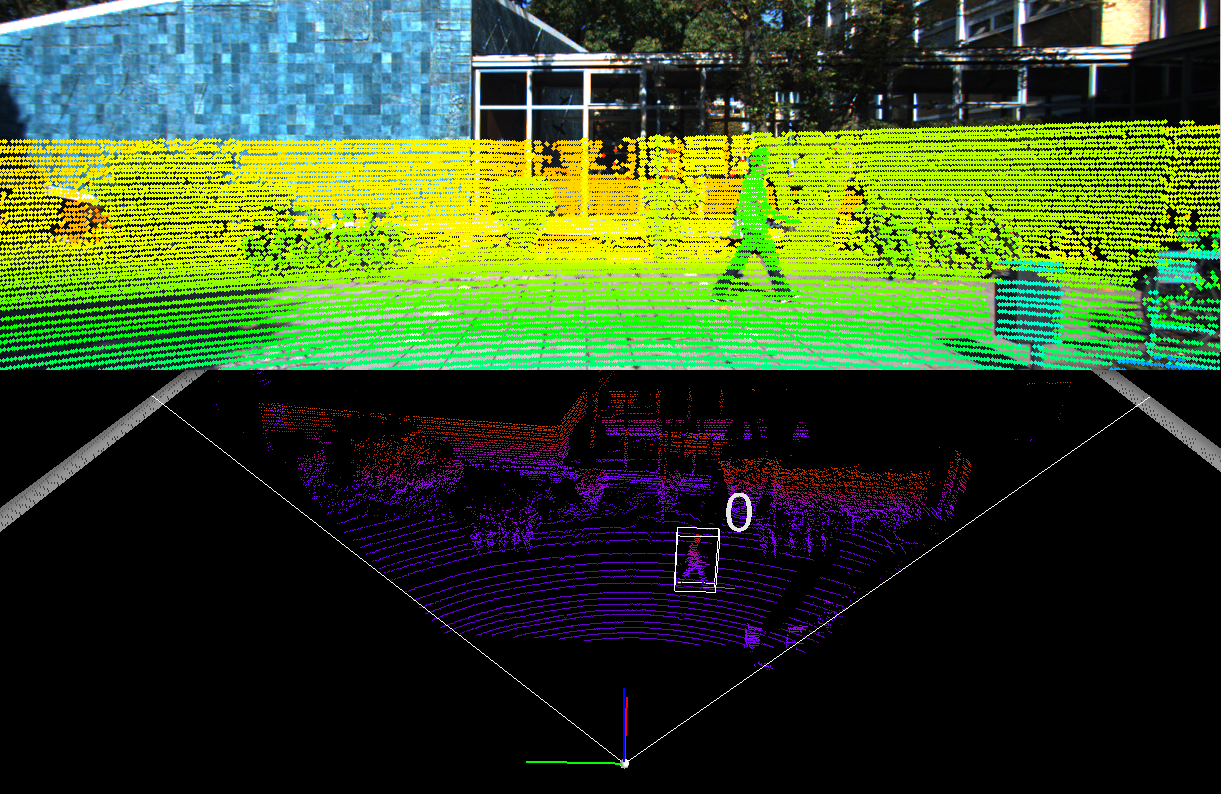

这些是直接运行F-Pointnets官方代码的结果:
aming@aming-All-Series:~/文档/Lidar/frustum-pointnets-master$ python kitti/prepare_data.py --demo
Type, truncation, occlusion, alpha: Pedestrian, 0, 0, -0.200000
2d bbox (x0,y0,x1,y1): 712.400000, 143.000000, 810.730000, 307.920000
3d bbox h,w,l: 1.890000, 0.480000, 1.200000
3d bbox location, ry: (1.840000, 1.470000, 8.410000), 0.010000
('Image shape: ', (370, 1224, 3))
 -------- 2D/3D bounding boxes in images --------
('pts_3d_extend shape: ', (8, 4))

 -------- LiDAR points and 3D boxes in velodyne coordinate --------
('All point num: ', 115384)
('FOV point num: ', 20285)
('pts_3d_extend shape: ', (8, 4))
('pts_3d_extend shape: ', (2, 4))

 -------- LiDAR points projected to image plane --------

 -------- LiDAR points in a 3D bounding box --------
('pts_3d_extend shape: ', (8, 4))
('Number of points in 3d box: ', 376)

 -------- LiDAR points in a frustum from a 2D box --------
[[1.8324e+01 4.9000e-02 8.2900e-01]
 [1.8344e+01 1.0600e-01 8.2900e-01]
 [5.1299e+01 5.0500e-01 1.9440e+00]
 [1.8317e+01 2.2100e-01 8.2900e-01]
 [1.8352e+01 2.5100e-01 8.3000e-01]
 [1.5005e+01 2.9400e-01 7.1700e-01]
 [1.4954e+01 3.4000e-01 7.1500e-01]
 [1.5179e+01 3.9400e-01 7.2300e-01]
 [1.8312e+01 5.3800e-01 8.2900e-01]
 [1.8300e+01 5.9500e-01 8.2800e-01]
 [1.8305e+01 6.2400e-01 8.2800e-01]
 [1.8305e+01 6.8200e-01 8.2900e-01]
 [1.8307e+01 7.3900e-01 8.2900e-01]
 [1.8301e+01 7.9700e-01 8.2900e-01]
 [1.8300e+01 8.5400e-01 8.2900e-01]
 [1.8287e+01 9.1100e-01 8.2800e-01]
 [1.8288e+01 9.6900e-01 8.2800e-01]
 [1.8307e+01 9.9900e-01 8.2900e-01]
 [1.8276e+01 1.0540e+00 8.2800e-01]
 [2.1017e+01 1.3490e+00 9.2100e-01]]
[[18.32401052  0.05322839  0.83005286]
 [18.34401095  0.11021263  0.83005313]
 [51.29900945  0.50918573  1.94510349]
 [18.31701048  0.22518075  0.83005276]
 [18.35201031  0.25517254  0.83105295]
 [15.00501117  0.29814455  0.71803507]
 [14.95401151  0.34412858  0.71603479]
 [15.17901091  0.39811201  0.72403614]
 [18.31201118  0.5420929   0.83005269]
 [18.30001012  0.59907705  0.82905281]
 [18.30501118  0.62806903  0.82905288]
 [18.30501115  0.68605293  0.83005259]
 [18.30701003  0.74303719  0.83005261]
 [18.30101139  0.80102102  0.83005253]
 [18.30001001  0.85800518  0.83005251]
 [18.28701141  0.91498924  0.82905263]
 [18.28801083  0.97297313  0.82905264]
 [18.30700992  1.00296512  0.83005261]
 [18.27600976  1.0579494   0.82905247]
 [21.01701075  1.35291567  0.92206282]]

 -------- LiDAR points in a frustum from a 2D box --------
('2d box FOV point num: ', 1483)
训练
CUDA_VISIBLE_DEVICES=1 sh scripts/command_train_v1.sh
...
 -- 2290 / 2294 --
mean loss: 1.606087
segmentation accuracy: 0.950418
box IoU (ground/3D): 0.797520 / 0.748949
box estimation accuracy (IoU=0.7): 0.756250
2019-12-01 13:51:22.648135
---- EPOCH 200 EVALUATION ----
eval mean loss: 4.188220
eval segmentation accuracy: 0.906205
eval segmentation avg class acc: 0.908660
eval box IoU (ground/3D): 0.747937 / 0.700035
eval box estimation accuracy (IoU=0.7): 0.640785
Model saved in file: train/log_v1/model.ckpt
4.1.2 准备训练数据
为了避免每次训练都花大量时间读取和预处理数据,这里首先基于2Dbox标签和2D检测器得到的box分别提取视锥点云和标签。
python kitti/prepare_data.py --gen_train --gen_val --gen_val_rgb_detection --car_only
4.1.3 跑一遍Frustum-Pointnets
CUDA_VISIBLE_DEVICES=0 sh scripts/command_train_v1.sh
CUDA_VISIBLE_DEVICES=0 sh scripts/command_test_v1.sh
这里默认使用2D groundtruth 进行测试,可以看到准确率(Moderate)为:
2D car 90.31 pedestrian 76.39 cyclist 72.70
bev car 82.60 pedestrian 63.26 cyclist 61.02
3D car 71.15 pedestrian 58.19 cyclist 58.84
Number of point clouds: 25392
Thank you for participating in our evaluation!
mkdir: 无法创建目录"train/detection_results_v1/plot": 文件已存在
Loading detections...
number of files for evaluation: 3769
  done.
save train/detection_results_v1/plot/car_detection.txt
car_detection AP: 96.482544 90.305161 87.626389
PDFCROP 1.38, 2012/11/02 - Copyright (c) 2002-2012 by Heiko Oberdiek.
==> 1 page written on `car_detection.pdf'.
save train/detection_results_v1/plot/pedestrian_detection.txt
pedestrian_detection AP: 84.555908 76.389679 72.438660
PDFCROP 1.38, 2012/11/02 - Copyright (c) 2002-2012 by Heiko Oberdiek.
==> 1 page written on `pedestrian_detection.pdf'.
save train/detection_results_v1/plot/cyclist_detection.txt
cyclist_detection AP: 88.994469 72.703659 70.610924
PDFCROP 1.38, 2012/11/02 - Copyright (c) 2002-2012 by Heiko Oberdiek.
==> 1 page written on `cyclist_detection.pdf'.
Finished 2D bounding box eval.
Going to eval ground for class: car
save train/detection_results_v1/plot/car_detection_ground.txt
car_detection_ground AP: 87.690544 82.598740 75.171814
PDFCROP 1.38, 2012/11/02 - Copyright (c) 2002-2012 by Heiko Oberdiek.
==> 1 page written on `car_detection_ground.pdf'.
Going to eval ground for class: pedestrian
save train/detection_results_v1/plot/pedestrian_detection_ground.txt
pedestrian_detection_ground AP: 72.566902 63.261135 57.889217
PDFCROP 1.38, 2012/11/02 - Copyright (c) 2002-2012 by Heiko Oberdiek.
==> 1 page written on `pedestrian_detection_ground.pdf'.
Going to eval ground for class: cyclist
save train/detection_results_v1/plot/cyclist_detection_ground.txt
cyclist_detection_ground AP: 82.455368 61.018501 57.501751
PDFCROP 1.38, 2012/11/02 - Copyright (c) 2002-2012 by Heiko Oberdiek.
==> 1 page written on `cyclist_detection_ground.pdf'.
Finished Birdeye eval.
Going to eval 3D box for class: car
save train/detection_results_v1/plot/car_detection_3d.txt
car_detection_3d AP: 83.958496 71.146927 63.374168
PDFCROP 1.38, 2012/11/02 - Copyright (c) 2002-2012 by Heiko Oberdiek.
==> 1 page written on `car_detection_3d.pdf'.
Going to eval 3D box for class: pedestrian
save train/detection_results_v1/plot/pedestrian_detection_3d.txt
pedestrian_detection_3d AP: 67.507156 58.191212 51.009769
PDFCROP 1.38, 2012/11/02 - Copyright (c) 2002-2012 by Heiko Oberdiek.
==> 1 page written on `pedestrian_detection_3d.pdf'.
Going to eval 3D box for class: cyclist
save train/detection_results_v1/plot/cyclist_detection_3d.txt
cyclist_detection_3d AP: 80.260239 58.842278 54.679943
PDFCROP 1.38, 2012/11/02 - Copyright (c) 2002-2012 by Heiko Oberdiek.
==> 1 page written on `cyclist_detection_3d.pdf'.
Finished 3D bounding box eval.
Your evaluation results are available at:
train/detection_results_v1
4.1.4 校准矩阵
calib/*.txt提供的校准矩阵分别是
- 校正后的投影矩阵(\(P^{(i)}_{rect} \in R^{3\times4}\))P0(左灰),P1(右灰),P2(左彩),P3(右彩)
- 校正旋转矩阵(\(R^(i) \in R^{3\times3}\)):R0_rect
- Tr_velo_to_cam
- Tr_imu_to_velo
P0: 7.070493000000e+02 0.000000000000e+00 6.040814000000e+02 0.000000000000e+00 0.000000000000e+00 7.070493000000e+02 1.805066000000e+02 0.000000000000e+00 0.000000000000e+00 0.000000000000e+00 1.000000000000e+00 0.000000000000e+00
P1: 7.070493000000e+02 0.000000000000e+00 6.040814000000e+02 -3.797842000000e+02 0.000000000000e+00 7.070493000000e+02 1.805066000000e+02 0.000000000000e+00 0.000000000000e+00 0.000000000000e+00 1.000000000000e+00 0.000000000000e+00
P2: 7.070493000000e+02 0.000000000000e+00 6.040814000000e+02 4.575831000000e+01 0.000000000000e+00 7.070493000000e+02 1.805066000000e+02 -3.454157000000e-01 0.000000000000e+00 0.000000000000e+00 1.000000000000e+00 4.981016000000e-03
P3: 7.070493000000e+02 0.000000000000e+00 6.040814000000e+02 -3.341081000000e+02 0.000000000000e+00 7.070493000000e+02 1.805066000000e+02 2.330660000000e+00 0.000000000000e+00 0.000000000000e+00 1.000000000000e+00 3.201153000000e-03
R0_rect: 9.999128000000e-01 1.009263000000e-02 -8.511932000000e-03 -1.012729000000e-02 9.999406000000e-01 -4.037671000000e-03 8.470675000000e-03 4.123522000000e-03 9.999556000000e-01
Tr_velo_to_cam: 6.927964000000e-03 -9.999722000000e-01 -2.757829000000e-03 -2.457729000000e-02 -1.162982000000e-03 2.749836000000e-03 -9.999955000000e-01 -6.127237000000e-02 9.999753000000e-01 6.931141000000e-03 -1.143899000000e-03 -3.321029000000e-01
Tr_imu_to_velo: 9.999976000000e-01 7.553071000000e-04 -2.035826000000e-03 -8.086759000000e-01 -7.854027000000e-04 9.998898000000e-01 -1.482298000000e-02 3.195559000000e-01 2.024406000000e-03 1.482454000000e-02 9.998881000000e-01 -7.997231000000e-01
坐标系有四个,分别是reference,rectified,image2和velodyne:
3d XYZ in
根据校准矩阵可以在坐标系之间相互投影,由于时间原因原理这里就不介绍了,而实现在Frustum-Pointnet/kitti/kitti_object/Calibration中非常详细,可以直接用。主要记住标签是rect camera coord的,所以都往这个坐标系做投影即可。
5. nuScenes
nuScenes没有2D box标签,需要生成。
KITTI虽然也有多个相机但benchmark是针对image_2能看见的物体进行评估,而nuScenes只有Lidar的benchmark,没有2D的benchmark,意味着如果要使用图像信息来参加nuScenes的3D目标检测测试集的评估,就必须六个图像都利用上,以此生成所有区域的检测结果。为了方便,这里先只考虑nuScenes的CAM_FRONT相机,自己划分trainval,不管test。
5.1 nuScenes转kitti
5.2 calibration
5.3 extract_frustum_data
'''
aming@aming-All-Series:~/文档/reproduced/frustum-pointnets-torch$ python nuscenes2kitti/prepare_data.py --gen_train --gen_val --car_only
--CAM_FRONT_only
...
------------- 7479
------------- 7480
Average pos ratio: 0.400264
Average npoints: 678.217072
'''
5.一些想法
能不能找些Car的3D CAD模型能否作为额外数据来改善kitti的3D目标检测性能, 毕竟kitti数据是真的少. 3D目标检测里好像还没人这么做.
6.环境说明
6.1 Pointnet
conda create -n torch1.3tf1.13cu100 python=3.7
source activate torch1.3tf1.13cu100
pip install --upgrade pip
pip install torch1.3.0+cu100 torchvision0.4.1+cu100 -f https://download.pytorch.org/whl/torch_stable.html
pip install h5py ipdb tqdm matplotlib plyfile imageio
pip install tensorboard
cd PointNet1_2_pytorch_repduced
CUDA_VISIBLE_DEVICES=0 python trainCls.py --name Default
tensorboard --logdir='./runscls'
(Then search localhost:6006)
6.2 Frustum-Pointnets
pip install tensorflow-gpu==1.13.1 #F-Pointnet官方代码用1.4,但1.4不支持CUDA10.0,参考这里 https://tensorflow.google.cn/install/source ,所以我装了1.13.1
pip install opencv-python
(follow the instruction in http://docs.enthought.com/mayavi/mayavi/installation.html#installing-with-pip to install mayavi
- download vtk https://vtk.org/download/#latest and compile:
unzip VTK
cd VTK
mkdir build
cd build
cmake ..
make
sudo make install - install mayavi and PyQt5
pip install mayavi
pip install PyQt5

 浙公网安备 33010602011771号