
CS231N Assignment3 入门笔记(Q1&Q2)
 斯坦福2023年春季CS231N课程第三次作业解析、笔记与代码,作为初学者入门学习。
斯坦福2023年春季CS231N课程第三次作业(最后一次)解析、笔记与代码,作为初学者入门学习。
在这项作业中,将实现语言网络,并将其应用于 COCO 数据集上的图像标题。然后将训练生成对抗网络,生成与训练数据集相似的图像。最后,您将学习自我监督学习,自动学习无标签数据集的视觉表示。
本作业的目标如下:
1.理解并实现 RNN 和 Transformer 网络。将它们与 CNN 网络相结合,为图像添加标题。
2.了解如何训练和实现生成对抗网络(GAN),以生成与数据集中的样本相似的图像。
3.了解如何利用自我监督学习技术来帮助完成图像分类任务。
Q1: Network Visualization: Saliency Maps, Class Visualization, and Fooling Images
The notebook Network_Visualization.ipynb will introduce the pretrained SqueezeNet model, compute gradients with respect to images, and use them to produce saliency maps and fooling images.
我们将探索使用image gradients来生成新图像。
在训练模型时,我们定义了一个损失函数来衡量我们目前对模型表现的不满。然后我们使用反向传播来计算损耗相对于模型参数的梯度,并对模型参数进行梯度下降以使损耗最小化。
在这里,我们将做一些略有不同的事情。我们将从一个CNN模型开始,该模型已经过预训练,可以在ImageNet数据集上执行图像分类。我们将使用这个模型来定义一个损失函数,它量化了我们当前对自己图像的不满。然后,我们将使用反向传播来计算这种损失相对于图像像素的梯度。然后,我们将保持模型不变,并对图像执行梯度下降,以合成一幅最大限度减少损失的新图像。
我们将探索三种图像生成技术:Saliency Maps、Fooling Images、 类别可视化Class Visualization
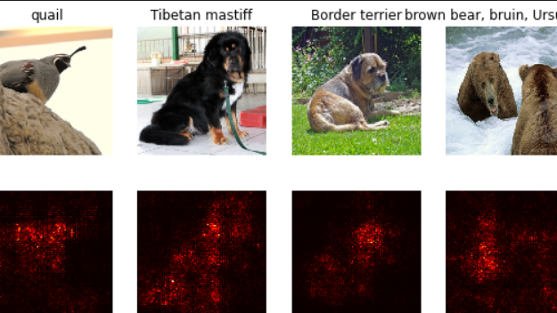
显著图Saliency Maps
可以使用显著图来判断图像的哪一部分影响了网络做出的分类决策。需要完成cs231n/net_visualization_pytorch.py当中的compute_saliency_maps函数
 1 def compute_saliency_maps(X, y, model):
 2     """
 3     Compute a class saliency map using the model for images X and labels y.
 4
 5     Input:
 6     - X: Input images; Tensor of shape (N, 3, H, W)
 7     - y: Labels for X; LongTensor of shape (N,)
 8     - model: A pretrained CNN that will be used to compute the saliency map.
 9
10     Returns:
11     - saliency: A Tensor of shape (N, H, W) giving the saliency maps for the input
12     images.
13     """
14     # Make sure the model is in "test" mode
15     # "test" mode下,模型通常会关闭一些训练中使用的特定层(如 dropout 或 batch normalization)
16     model.eval()
17
18     # Make input tensor require gradient
19     # 告诉 PyTorch 在计算模型的前向传播时跟踪输入图像 X 的梯度。
20     X.requires_grad_()
21
22     saliency = None
23     ##############################################################################
24     # TODO: Implement this function. Perform a forward and backward pass through #
25     # the model to compute the gradient of the correct class score with respect  #
26     # to each input image. You first want to compute the loss over the correct   #
27     # scores (we'll combine losses across a batch by summing), and then compute  #
28     # the gradients with a backward pass.                                        #
29     ##############################################################################
30     # *****START OF YOUR CODE (DO NOT DELETE/MODIFY THIS LINE)*****
31
32     # 执行Forward pass
33     scores = model(X)
34     # y.view(-1, 1) 将标签 y 变形为列向量
35     # 使用 gather(1,) 从 scores 中选择正确类别的分数
36     correct_scores = scores.gather(1, y.view(-1, 1))
37     # Compute loss
38     # 使用负的正确类别分数的和作为损失,因为我们想要最大化这个分数。
39     loss = -correct_scores.sum()
40
41     # 执行Backward pass
42     loss.backward()
43     # Compute the saliency map
44     # 梯度.绝对值.三通道当中的最大值,dim=1即对应(N, 3, H, W)的3
45     # 注意若没有[0],则第一个张量是最大值的张量,第二个张量是对应最大值的索引。
46     saliency = X.grad.abs().max(dim=1)[0]
47
48     # Clear gradients for next iteration
49     # 清零输入图像的梯度,以确保下一次迭代时梯度不会累积。
50     X.grad.data.zero_()
51
52     # *****END OF YOUR CODE (DO NOT DELETE/MODIFY THIS LINE)*****
53     ##############################################################################
54     #                             END OF YOUR CODE                               #
55     ##############################################################################
56     return saliency
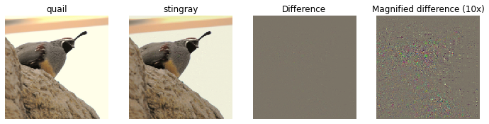
Fooling Images
可以干扰输入图像,使其在人类看来是相同的,但会被预先训练的网络错误分类。需要完成cs231n/net_visualization_pytorch.py当中的make_fooling_image函数
 1 def make_fooling_image(X, target_y, model):
 2     """
 3     Generate a fooling image that is close to X, but that the model classifies
 4     as target_y.
 5
 6     Inputs:
 7     - X: Input image; Tensor of shape (1, 3, 224, 224)
 8     - target_y: An integer in the range [0, 1000)
 9     - model: A pretrained CNN
10
11     Returns:
12     - X_fooling: An image that is close to X, but that is classifed as target_y
13     by the model.
14     """
15     # Initialize our fooling image to the input image, and make it require gradient
16     X_fooling = X.clone()
17     X_fooling = X_fooling.requires_grad_()
18
19     learning_rate = 1
20     ##############################################################################
21     # TODO: Generate a fooling image X_fooling that the model will classify as   #
22     # the class target_y. You should perform gradient ascent on the score of the #
23     # target class, stopping when the model is fooled.                           #
24     # When computing an update step, first normalize the gradient:               #
25     #   dX = learning_rate * g / ||g||_2                                         #
26     #                                                                            #
27     # You should write a training loop.                                          #
28     #                                                                            #
29     # HINT: For most examples, you should be able to generate a fooling image    #
30     # in fewer than 100 iterations of gradient ascent.                           #
31     # You can print your progress over iterations to check your algorithm.       #
32     ##############################################################################
33     # *****START OF YOUR CODE (DO NOT DELETE/MODIFY THIS LINE)*****
34
35     # Set the model to evaluation mode
36     model.eval()
37
38     # Define a criterion (loss function) to maximize the target class score
39     # criterion = torch.nn.CrossEntropyLoss()
40
41     #初始分类
42     scores = model(X_fooling)
43
44     _, y_predit = scores.max(dim = 1)
45
46     iter = 0
47
48     while(y_predit != target_y):
49         iter += 1
50
51         target_score = scores[0, target_y]
52         target_score.backward()
53         grad = X_fooling.grad / X_fooling.grad.norm()
54         X_fooling.data += learning_rate * grad
55
56         X_fooling.grad.zero_()
57
58         model.zero_rgrad()
59
60         scores = model(X_fooling)
61         _,y_predit=scores.max(dim = 1)
62
63     print("Iteration Count: %d"% iter)
64
65
66     # *****END OF YOUR CODE (DO NOT DELETE/MODIFY THIS LINE)*****
67     ##############################################################################
68     #                             END OF YOUR CODE                               #
69     ##############################################################################
70     return X_fooling
例如idx = 1,target_y = 6,输出为
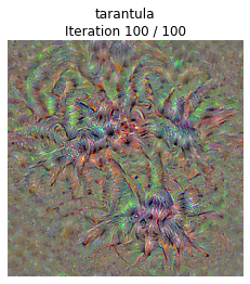
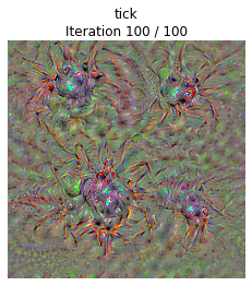
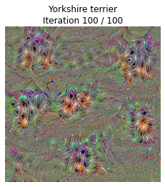
类别可视化Class Visualization
可以合成图像以最大化特定类别的分类分数;这可以让我们对网络在对该类别的图像进行分类时寻找什么有所了解。
 1 def class_visualization_update_step(img, model, target_y, l2_reg, learning_rate):
 2     ########################################################################
 3     # TODO: Use the model to compute the gradient of the score for the     #
 4     # class target_y with respect to the pixels of the image, and make a   #
 5     # gradient step on the image using the learning rate. Don't forget the #
 6     # L2 regularization term!                                              #
 7     # Be very careful about the signs of elements in your code.            #
 8     ########################################################################
 9     # *****START OF YOUR CODE (DO NOT DELETE/MODIFY THIS LINE)*****
10
11     score = model(img)
12     target_score = score[0,target_y]
13     target_score.backward()
14
15     im_grad = img.grad - l2_reg * img
16     grad = im_grad / im_grad.norm()
17     img.data += learning_rate * grad
18     img.grad.zero_()
19     model.zero_grad()
20
21     # *****END OF YOUR CODE (DO NOT DELETE/MODIFY THIS LINE)*****
22     ########################################################################
23     #                             END OF YOUR CODE                         #
24     ########################################################################
25
26 def create_class_visualization(target_y, model, dtype, **kwargs):
27     """
28     Generate an image to maximize the score of target_y under a pretrained model.
29
30     Inputs:
31     - target_y: Integer in the range [0, 1000) giving the index of the class
32     - model: A pretrained CNN that will be used to generate the image
33     - dtype: Torch datatype to use for computations
34
35     Keyword arguments:
36     - l2_reg: Strength of L2 regularization on the image
37     - learning_rate: How big of a step to take
38     - num_iterations: How many iterations to use
39     - blur_every: How often to blur the image as an implicit regularizer
40     - max_jitter: How much to gjitter the image as an implicit regularizer
41     - show_every: How often to show the intermediate result
42     """
43     model.type(dtype)
44
45     l2_reg = kwargs.pop('l2_reg', 1e-3)
46     learning_rate = kwargs.pop('learning_rate', 25)
47     num_iterations = kwargs.pop('num_iterations', 100)
48     blur_every = kwargs.pop('blur_every', 10)
49     max_jitter = kwargs.pop('max_jitter', 16)
50     show_every = kwargs.pop('show_every', 25)
51
52     # 随机初始化生成图像,其数据类型为 dtype,并标记为需要梯度计算
53     img = torch.randn(1, 3, 224, 224).mul_(1.0).type(dtype).requires_grad_()
54
55     for t in range(num_iterations):
56         # 在每次迭代中,随机对图像进行轻微的抖动,这是为了得到稍微更好的结果。
57         ox, oy = random.randint(0, max_jitter), random.randint(0, max_jitter)
58         img.data.copy_(jitter(img.data, ox, oy))
59         class_visualization_update_step(img, model, target_y, l2_reg, learning_rate)
60         # 恢复图像,撤销之前的抖动。
61         img.data.copy_(jitter(img.data, -ox, -oy))
62
63         # As regularizer, clamp and periodically blur the image
64         for c in range(3):
65             lo = float(-SQUEEZENET_MEAN[c] / SQUEEZENET_STD[c])
66             hi = float((1.0 - SQUEEZENET_MEAN[c]) / SQUEEZENET_STD[c])
67             img.data[:, c].clamp_(min=lo, max=hi)
68         # 每隔一定的迭代次数对图像进行模糊处理
69         if t % blur_every == 0:
70             blur_image(img.data, sigma=0.5)
71
72         # Periodically show the image
73         if t == 0 or (t + 1) % show_every == 0 or t == num_iterations - 1:
74             plt.imshow(deprocess(img.data.clone().cpu()))
75             class_name = class_names[target_y]
76             plt.title('%s\nIteration %d / %d' % (class_name, t + 1, num_iterations))
77             plt.gcf().set_size_inches(4, 4)
78             plt.axis('off')
79             plt.show()
80
81     return deprocess(img.data.cpu())

net_visualizaiton_pytorch.py还附上了抖动之类的函数,解析如下:
 1 def jitter(X, ox, oy):
 2     """
 3     Helper function to randomly jitter an image.
 4
 5     Inputs
 6     - X: PyTorch Tensor of shape (N, C, H, W)
 7     - ox, oy: Integers giving number of pixels to jitter along W and H axes
 8
 9     Returns: A new PyTorch Tensor of shape (N, C, H, W)
10     """
11     # 如果 ox 不等于零,表示需要在图像的水平方向进行抖动,
12     # 将图像沿着水平方向切分成两部分,然后将右侧的部分移动到左侧。
13     if ox != 0:
14         left = X[:, :, :, :-ox]
15         right = X[:, :, :, -ox:]
16         X = torch.cat([right, left], dim=3)
17     # 如果 oy 不等于零,表示需要在图像的垂直方向进行抖动,
18     # 将图像沿着垂直方向切分成两部分,然后将上侧的部分移动到下侧。
19     if oy != 0:
20         top = X[:, :, :-oy]
21         bottom = X[:, :, -oy:]
22         X = torch.cat([bottom, top], dim=2)
23     return X
高斯模糊处理函数
注意转换成了numpy数组进行了处理,再转换回pytorch张量。
1 def blur_image(X, sigma=1):
2     X_np = X.cpu().clone().numpy() # 转换成numpy数组
3     X_np = gaussian_filter1d(X_np, sigma, axis=2) # 水平方向
4     X_np = gaussian_filter1d(X_np, sigma, axis=3) # 垂直方向
5     X.copy_(torch.Tensor(X_np).type_as(X)) # 转换为pytorch张量
6     return X
Q2: Image Captioning with Vanilla RNNs
The notebook RNN_Captioning.ipynb will walk you through the implementation of vanilla recurrent neural networks and apply them to image captioning on COCO.
Inspect the Data的时候有可能会报错,重新运行就OK了。
Step Forward前向传播
1 def rnn_step_forward(x, prev_h, Wx, Wh, b):
2
3     next_h, cache = None, None
4
5     next_h = np.tanh(x.dot(Wx) + prev_h.dot(Wh) + b)
6     cache = (next_h, x, Wx, prev_h, Wh, b)
7
8     return next_h, cache
Step Backward后向传播
1 def rnn_step_backward(dnext_h, cache):
2
3 dx, dprev_h, dWx, dWh, db = None, None, None, None, None
4
5 next_h, x, Wx, prev_h, Wh, b = cache
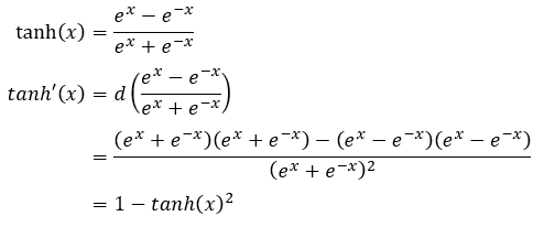
6 # next_h = np.tanh(x.dot(Wx) + prev_h.dot(Wh) + b)
7 dtanh = dnext_h * (1 - next_h ** 2)
8
9 # x = np.random.randn(N, D),转置后(D,N) * (N,H)
10 dWx = x.T.dot(dtanh)
11 # (H,N) * (N,H)
12 dWh = prev_h.T.dot(dtanh)
13
14 dprev_h = dtanh.dot(Wh.T) # (N,H) * (H,H)= (N,H)
15
16 dx = dtanh.dot(Wx.T) # (N,H)*(H,D)=(N,D)
17 # 偏置项 b 的梯度为按列求和。
18 db = np.sum(dtanh, axis=0)
19
20 return dx, dprev_h, dWx, dWh, db
RNN前向传播
def rnn_forward(x, h0, Wx, Wh, b):

    h, cache = None, None

    # x: (N, T, D)
    # ht:(N,    H)
    # h:  (N, T, H)
    N, T, D = x.shape
    ht = h0
    h = np.zeros((N, T, h0.shape[1]))
    cache = []
    for t in range(T):
        # def rnn_step_forward(x, prev_h, Wx, Wh, b):
        #   return next_h, cache
        ht, cache_step = rnn_step_forward(x[:, t, :], ht, Wx, Wh, b)
        h[:, t, :] = ht
        cache.append(cache_step)

    return h, cache
RNN后向传播
def rnn_backward(dh, cache):

    dx, dh0, dWx, dWh, db = None, None, None, None, None

    # h:  (N, T, H)
    # dh:  (N, T, H)
    N, T, H = dh.shape
    # 此外还需要一个D的数据,鉴于传入的参数只有dh和cache
    # cache = (next_h, x, Wx, prev_h, Wh, b)
    # 可以考虑cache中x的第二个维度或者Wx的第0个维度
    # 例如利用Wx,取cache的0行的第2个元素Wx的第0个维度:
    # (具体参数需要参考之前step forward当中cache的设定)
    D = cache[0][2].shape[0]

    dx = np.zeros((N, T, D))
    dh0 = np.zeros((N, H))

    dWx = np.zeros((D, H))
    dWh = np.zeros((H, H))
    db = np.zeros((H,))
    # T时刻dpre_h初始化
    dprev_h = np.zeros((N, H))

    for t in reversed(range(T)): # 注意这里reversed
        # 加上t+1时刻传来的dh
        dnext_h = dh[:, t, :] + dprev_h

        # def rnn_step_backward(dnext_h, cache):
        #   return dx, dprev_h, dWx, dWh, db

        # 这里也看到有代码写的是pop一个缓存
        # dx[:, t, :], dprev_h, dWx_t, dWh_t, db_t = rnn_step_backward(dnext_h, cache[t])
        dx[:, t, :], dprev_h, dWx_t, dWh_t, db_t = rnn_step_backward(dnext_h, cache[t])
        # 均为累加
        dWx += dWx_t
        dWh += dWh_t
        db += db_t

    dh0 = dprev_h

    return dx, dh0, dWx, dWh, db
Word Embedding
前向
1 def word_embedding_forward(x, W):
2
3     out, cache = None, None
4
5     out = W[x]
6     cache = (x, W)
7
8
9     return out, cache
以作业中的数据为例:
x: (N, T)
[[0 3 1 2]
[2 1 0 3]]
W: (V, D)
[[0.0000000 0.07142857 0.14285714]
[0.21428571 0.28571429 0.35714286]
[0.42857143 0.50000000 0.57142857]
[0.64285714 0.71428571 0.78571429]
[0.85714286 0.92857143 1. 0000000]]
out: (N, T, D)
[[[0.00000000 0.07142857 0.14285714]
[0.64285714 0.71428571 0.78571429]
[0.21428571 0.28571429 0.35714286]
[0.42857143 0.50000000 0.57142857]]
[[0.42857143 0.50000000 0.57142857]
[0.21428571 0.28571429 0.35714286]
[0.00000000 0.07142857 0.14285714]
[0.64285714 0.71428571 0.78571429]]]
后向传递要用dout和cache里的x和W计算dW
把参数改小了一些方便参考:
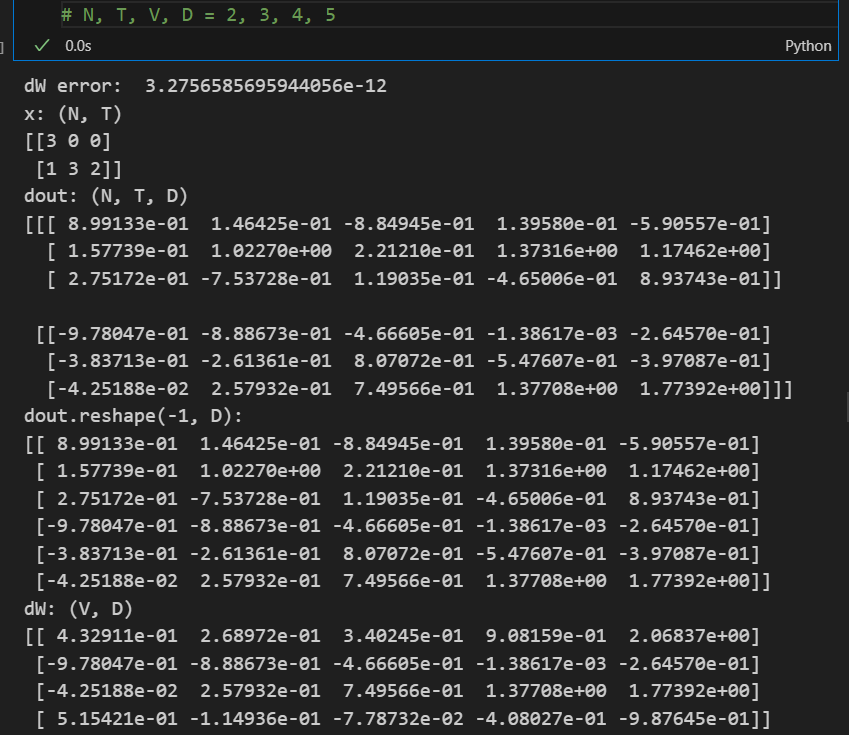
注意此时x化成了一维数组,dout按D化成了二维数组方便读取,对比dW的1、2元素和0、3元素,注意到在dW进行0初始化之后,np.add可以方便地实现原地相加。
 1 def word_embedding_backward(dout, cache):
 2
 3     dW = None
 4
 5     x, W = cache
 6     N, T, D = dout.shape
 7     dW = np.zeros(W.shape)
 8     np.add.at(dW, x.flatten(), dout.reshape(-1, D))
 9
10     return dW
Temporal Affine Layer时间仿射层
  1 def temporal_affine_forward(x, w, b):
  2     """Forward pass for a temporal affine layer.
  3
  4     The input is a set of D-dimensional
  5     vectors arranged into a minibatch of N timeseries,
  6     each of length T. We use
  7     an affine function to transform each of those vectors into a new vector of
  8     dimension M.
  9
 10
 11     Inputs:
 12     - x: Input data of shape (N, T, D)
 13     - w: Weights of shape (D, M)
 14     - b: Biases of shape (M,)
 15
 16     Returns a tuple of:
 17     - out: Output data of shape (N, T, M)
 18     - cache: Values needed for the backward pass
 19     """
 20     N, T, D = x.shape
 21     M = b.shape[0]
 22     out = x.reshape(N * T, D).dot(w).reshape(N, T, M) + b
 23     cache = x, w, b, out
 24     return out, cache
 25
 26
 27 def temporal_affine_backward(dout, cache):
 28     """Backward pass for temporal affine layer.
 29
 30     Input:
 31     - dout: Upstream gradients of shape (N, T, M) 上游梯度
 32     - cache: Values from forward pass
 33
 34     Returns a tuple of:
 35     - dx: Gradient of input, of shape (N, T, D)
 36     - dw: Gradient of weights, of shape (D, M)
 37     - db: Gradient of biases, of shape (M,)
 38     """
 39     x, w, b, out = cache
 40     N, T, D = x.shape
 41     M = b.shape[0]
 42
 43     dx = dout.reshape(N * T, M).dot(w.T).reshape(N, T, D)
 44     dw = dout.reshape(N * T, M).T.dot(x.reshape(N * T, D)).T
 45     db = dout.sum(axis=(0, 1)) #先沿着0方向求和,再沿着1方向求和
 46
 47     return dx, dw, db
 48
 49
 50 def temporal_softmax_loss(x, y, mask, verbose=False):
 51     """A temporal version of softmax loss for use in RNNs.
 52
 53     We assume that we are making predictions over a vocabulary of size V for each timestep of a
 54     timeseries of length T, over a minibatch of size N. The input x gives scores for all vocabulary
 55     elements at all timesteps, and y gives the indices of the ground-truth element at each timestep.
 56     We use a cross-entropy loss at each timestep, summing the loss over all timesteps and averaging
 57     across the minibatch.
 58
 59     As an additional complication, we may want to ignore the model output at some timesteps, since
 60     sequences of different length may have been combined into a minibatch and padded with NULL
 61     tokens. The optional mask argument tells us which elements should contribute to the loss.
 62
 63     Inputs:
 64     - x: Input scores, of shape (N, T, V)
 65     - y: Ground-truth indices, of shape (N, T) where each element is in the range
 66          0 <= y[i, t] < V
 67     - mask: Boolean array of shape (N, T) where mask[i, t] tells whether or not
 68       the scores at x[i, t] should contribute to the loss.
 69
 70     Returns a tuple of:
 71     - loss: Scalar giving loss
 72     - dx: Gradient of loss with respect to scores x.
 73     """
 74
 75     N, T, V = x.shape
 76
 77     x_flat = x.reshape(N * T, V) # x二维数组
 78     y_flat = y.reshape(N * T) # y一维数组
 79     mask_flat = mask.reshape(N * T) # mask一维数组
 80
 81     probs = np.exp(x_flat - np.max(x_flat, axis=1, keepdims=True))
 82     probs /= np.sum(probs, axis=1, keepdims=True)
 83
 84     # 使用掩码矩阵 mask_flat 对概率矩阵 probs 进行筛选
 85     # 只保留需要参与损失计算的位置。
 86     # 即使用索引数组 np.arange(N * T) 和真实标签数组 y_flat
 87     # 来获取每个样本在概率矩阵中对应位置的概率,并取对数。
 88     # 最后,将这些对数概率乘以掩码矩阵,
 89     # 并对所有样本的损失求和并除以小批量大小 N,得到平均损失。
 90     loss = -np.sum(mask_flat * np.log(probs[np.arange(N * T), y_flat])) / N
 91
 92     dx_flat = probs.copy()
 93     # 使用索引数组 np.arange(N * T) 和真实标签数组 y_flat,
 94     # 可以定位到每个样本在概率矩阵中对应位置的概率,
 95     # 并将这些位置上的值减去 1。
 96     dx_flat[np.arange(N * T), y_flat] -= 1
 97     dx_flat /= N
 98     # 将梯度矩阵 dx_flat 乘以掩码矩阵 mask_flat 的转置。
 99     # 只有掩码为真的位置上的梯度才会保留,其他位置上的梯度都被置为零。
100     dx_flat *= mask_flat[:, None]
101
102     if verbose:
103         print("dx_flat: ", dx_flat.shape)
104
105     dx = dx_flat.reshape(N, T, V)
106
107     return loss, dx
RNN for Image Captioning
首先实现loss函数,基本就是照着提示1-5写即可
 1 def loss(self, features, captions):
 2         """
 3         Compute training-time loss for the RNN. We input image features and
 4         ground-truth captions for those images, and use an RNN (or LSTM) to compute
 5         loss and gradients on all parameters.
 6
 7         Inputs:
 8         - features: Input image features, of shape (N, D)
 9         - captions: Ground-truth captions; an integer array of shape (N, T + 1) where
10           each element is in the range 0 <= y[i, t] < V
11
12         Returns a tuple of:
13         - loss: Scalar loss
14         - grads: Dictionary of gradients parallel to self.params
15         """
16         # Cut captions into two pieces: captions_in has everything but the last word
17         # and will be input to the RNN; captions_out has everything but the first
18         # word and this is what we will expect the RNN to generate. These are offset
19         # by one relative to each other because the RNN should produce word (t+1)
20         # after receiving word t. The first element of captions_in will be the START
21         # token, and the first element of captions_out will be the first word.
22         captions_in = captions[:, :-1] #除了最后一列
23         captions_out = captions[:, 1:] #除了第一列
24
25         # 生成一个用来忽略<NULL>的布尔数组作为掩码
26         # True表示该处不为<NULL>
27         mask = captions_out != self._null
28
29         # Weight and bias for the affine transform from image features to initial
30         # hidden state
31         W_proj, b_proj = self.params["W_proj"], self.params["b_proj"]
32
33         # Word embedding matrix
34         W_embed = self.params["W_embed"]
35
36         # Input-to-hidden, hidden-to-hidden, and biases for the RNN
37         Wx, Wh, b = self.params["Wx"], self.params["Wh"], self.params["b"]
38
39         # Weight and bias for the hidden-to-vocab transformation.
40         W_vocab, b_vocab = self.params["W_vocab"], self.params["b_vocab"]
41
42         loss, grads = 0.0, {}
43         ############################################################################
44         # TODO: Implement the forward and backward passes for the CaptioningRNN.   #
45         # In the forward pass you will need to do the following:                   #
46         # (1) Use an affine transformation to compute the initial hidden state     #
47         #     from the image features. This should produce an array of shape (N, H)#
48         # 使用仿射变换(affine)从图像特征计算初始隐藏状态h0,得到形状为(N,H)的数组
49         h0, cache_affine = affine_forward(features, W_proj, b_proj)
50         # (2) Use a word embedding layer to transform the words in captions_in     #
51         #     from indices to vectors, giving an array of shape (N, T, W).         #
52         # 使用词嵌入层(word embedding)将captions_in中的单词从索引转换为向量,得到形状为(N,T,W)的数组。
53         x, cache_embed = word_embedding_forward(captions_in, W_embed)
54         # (3) Use either a vanilla RNN or LSTM (depending on self.cell_type) to    #
55         #     process the sequence of input word vectors and produce hidden state  #
56         #     vectors for all timesteps, producing an array of shape (N, T, H).    #
57         if self.cell_type == 'rnn':
58             h, cache_rnn = rnn_forward(x, h0, Wx, Wh, b)
59         elif self.cell_type == 'lstm':
60             h, cache_rnn = lstm_forward(x, h0, Wx, Wh, b)
61         # (4) Use a (temporal) affine transformation to compute scores over the    #
62         #     vocabulary at every timestep using the hidden states, giving an      #
63         #     array of shape (N, T, V).                                            #
64         scores, cache_scores = temporal_affine_forward(h, W_vocab, b_vocab)
65         # (5) Use (temporal) softmax to compute loss using captions_out, ignoring  #
66         #     the points where the output word is <NULL> using the mask above.     #
67         loss, dx = temporal_softmax_loss(scores, captions_out, mask)
68
69         # In the backward pass you will need to compute the gradient of the loss   #
70         # with respect to all model parameters. Use the loss and grads variables   #
71         # defined above to store loss and gradients; grads[k] should give the      #
72         # gradients for self.params[k].                                            #
73         # (4)
74         dx, grads['W_vocab'], grads['b_vocab'] = temporal_affine_backward(dx, cache_scores)
75         # (3)
76         if self.cell_type == 'rnn':
77             dx, dh, grads['Wx'], grads['Wh'], grads['b'] = rnn_backward(dx, cache_rnn)
78         elif self.cell_type == 'lstm':
79             dx, dh, grads['Wx'], grads['Wh'], grads['b'] = lstm_backward(dx, cache_rnn)
80         # (2)
81         grads['W_embed'] = word_embedding_backward(dx, cache_embed)
82         # (1)
83         dh0, grads['W_proj'], grads['b_proj'] = affine_backward(dh, cache_affine)
84
85         return loss, grads
Overfit RNN Captioning Model on Small Data
num_batches = N / batch_size
# 这里可能要改成
num_batches = N // batch_size
RNN Sampling at Test Time
与分类模型不同,图像字幕模型在训练与测试时的行为有较大差异。在训练时间,我们可以直接获取标题,在每个timestep中将标题作为输入传给RNN。在测试时,我们从每个timestep的词汇表分布中进行采样,并在下一个timestep将采样样本作为输入提供给RNN。
在`cs231n/classifiers/rnn.py`文件中,实现测试时间采样的`sample`方法。执行此操作后,运行以下命令以从训练和验证数据的过拟合模型中进行采样。训练数据上的样本应该是非常好的。然而,验证数据上的样本可能没有意义。
 1 def sample(self, features, max_length=30):
 2         """
 3         Run a test-time forward pass for the model, sampling captions for input
 4         feature vectors.
 5
 6         At each timestep, we embed the current word, pass it and the previous hidden
 7         state to the RNN to get the next hidden state, use the hidden state to get
 8         scores for all vocab words, and choose the word with the highest score as
 9         the next word. The initial hidden state is computed by applying an affine
10         transform to the input image features, and the initial word is the <START>
11         token.
12         在每个时间步,我们嵌入当前单词,将当前单词和先前的隐藏状态传递给RNN,以获得下一个
13         隐藏状态,使用该隐藏状态获得所有单词的分数,并选择得分最高的单词作为下一个单词。
14         初始隐藏状态是通过对输入图像特征应用仿射变换来计算的,初始单词是<Start>标记。
15
16         For LSTMs you will also have to keep track of the cell state; in that case
17         the initial cell state should be zero.
18         对于LSTM,您还必须跟踪单元状态;在这种情况下,初始单元状态应该为零。
19
20         Inputs:
21         - features: Array of input image features of shape (N, D).
22         - max_length: Maximum length T of generated captions.
23
24         Returns:
25         - captions: Array of shape (N, max_length) giving sampled captions,
26           where each element is an integer in the range [0, V). The first element
27           of captions should be the first sampled word, not the <START> token.
28         """
29         N = features.shape[0]
30         captions = self._null * np.ones((N, max_length), dtype=np.int32)
31
32         # Unpack parameters
33         W_proj, b_proj = self.params["W_proj"], self.params["b_proj"]
34         W_embed = self.params["W_embed"]
35         Wx, Wh, b = self.params["Wx"], self.params["Wh"], self.params["b"]
36         W_vocab, b_vocab = self.params["W_vocab"], self.params["b_vocab"]
37
38         ###########################################################################
39         # TODO: Implement test-time sampling for the model. You will need to      #
40         # initialize the hidden state of the RNN by applying the learned affine   #
41         # transform to the input image features. The first word that you feed to  #
42         # the RNN should be the <START> token; its value is stored in the         #
43         # variable self._start.                                                   #
44         # For simplicity, you do not need to stop generating after an <END> token #
45         # is sampled, but you can if you want to.                                 #
46         #                                                                         #
47         # HINT: You will not be able to use the rnn_forward or lstm_forward       #
48         # functions; you'll need to call rnn_step_forward or lstm_step_forward in #
49         # a loop.                                                                 #
50         #                                                                         #
51         # NOTE: we are still working over minibatches in this function. Also if   #
52         # you are using an LSTM, initialize the first cell state to zeros.        #
53         ###########################################################################
54         # 初始化
55         h0, _ = affine_forward(features, W_proj, b_proj)
56         ht = h0
57
58         # 创建一个形状为(N,)的数组word,并将其所有元素设置为起始标记<START>的索引值。
59         word = self._start * np.ones((N,), dtype=np.int32)
60
61         for i in range(max_length):
62             # (1) Embed the previous word using the learned word embeddings
63             x, _ = word_embedding_forward(word, W_embed)
64             # (2) Make an RNN step using the previous hidden state and the embedded
65             #     current word to get the next hidden state.
66
67             if self.cell_type == 'rnn':
68                 ht, _ = rnn_step_forward(x, ht, Wx, Wh, b)
69             else:
70                 ht, next_c, _ = lstm_step_forward(x, ht, next_c, Wx, Wh, b)
71             # (3) Apply the learned affine transformation to the next hidden state to #
72             #     get scores for all words in the vocabulary
73             scores, _ = affine_forward(ht, W_vocab, b_vocab)
74             # (4) Select the word with the highest score as the next word, writing it #
75             #     (the word index) to the appropriate slot in the captions variable   #
76             word_predict = scores.argmax(1)
77             captions[:, i] = word_predict
78         return captions
参考:https://github.com/hanlulu1998/CS231n/tree/master/assignment3

 浙公网安备 33010602011771号