不同阻尼比下的振动形式-python代码

import numpy as np
import matplotlib.pyplot as plt

# 定义参数
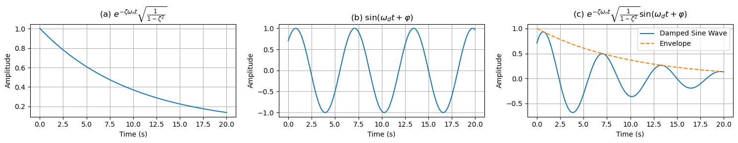
zeta = 0.1  # 阻尼比减小，以实现更慢的衰减
omega_n = 1.0  # 自然频率
omega_d = omega_n * np.sqrt(1 - zeta**2)  # 阻尼频率
varphi = np.pi / 4  # 相位角

# 定义时间变量
t = np.linspace(0, 20, 2000)  # 从0到20秒，2000个点，增加周期

# 计算函数值
a = np.exp(-zeta * omega_n * t) * np.sqrt(1 / (1 - zeta**2))
b = np.sin(omega_d * t + varphi)
c = np.exp(-zeta * omega_n * t) * np.sqrt(1 / (1 - zeta**2)) * np.sin(omega_d * t + varphi)

# 绘制图像
plt.figure(figsize=(15, 5))  # 设置整个图像的大小

# 绘制(a)部分
plt.subplot(1, 3, 1)  # 1行3列的第1个
plt.plot(t, a)
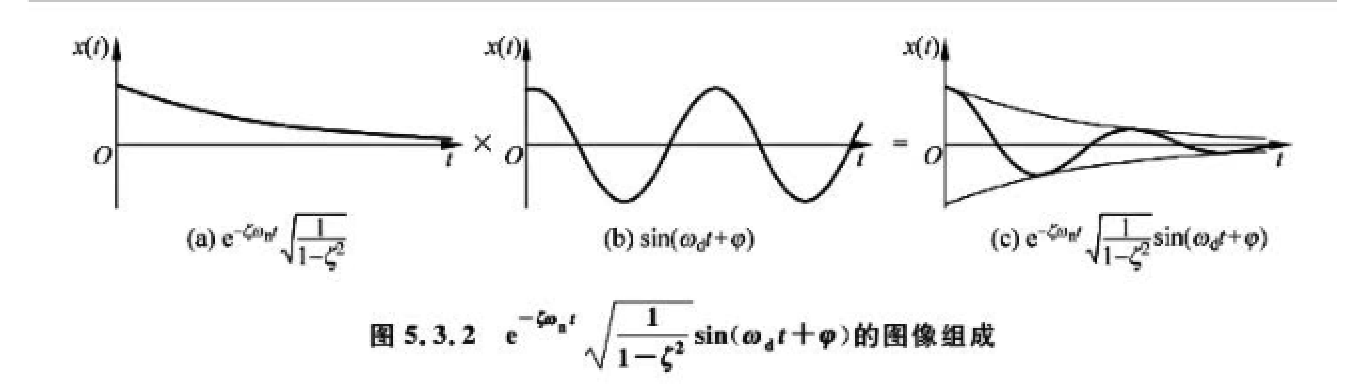
plt.title(r'(a) $e^{-\zeta\omega_{n} t}\sqrt{\frac{1}{1-\zeta^2}}$')
plt.xlabel('Time (s)')
plt.ylabel('Amplitude')
plt.grid(True)

# 绘制(b)部分
plt.subplot(1, 3, 2)  # 1行3列的第2个
plt.plot(t, b)
plt.title(r'(b) $\sin(\omega_{d} t+\varphi)$')
plt.xlabel('Time (s)')
plt.ylabel('Amplitude')
plt.grid(True)

# 绘制(c)部分
plt.subplot(1, 3, 3)  # 1行3列的第3个
plt.plot(t, c, label='Damped Sine Wave')
plt.plot(t, a, label='Envelope', linestyle='--')  # 绘制包络线
plt.title(r'(c) $e^{-\zeta\omega_{n} t}\sqrt{\frac{1}{1-\zeta^2}}\sin(\omega_{d} t+\varphi)$')
plt.xlabel('Time (s)')
plt.ylabel('Amplitude')
plt.legend()
plt.grid(True)

# 显示图像
plt.tight_layout()  # 调整子图间距
plt.show()

import numpy as np
import matplotlib.pyplot as plt

# 定义参数
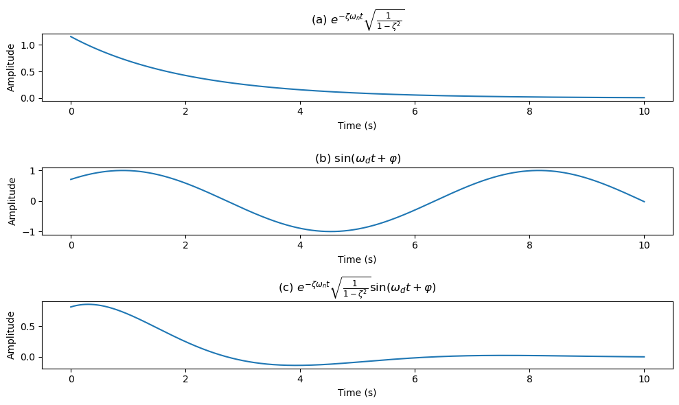
zeta = 0.5  # 阻尼比
omega_n = 1.0  # 自然频率
omega_d = omega_n * np.sqrt(1 - zeta**2)  # 阻尼频率
varphi = np.pi / 4  # 相位角

# 定义时间变量
t = np.linspace(0, 10, 1000)  # 从0到10秒，1000个点

# 计算函数值
a = np.exp(-zeta * omega_n * t) * np.sqrt(1 / (1 - zeta**2))
b = np.sin(omega_d * t + varphi)
c = np.exp(-zeta * omega_n * t) * np.sqrt(1 / (1 - zeta**2)) * np.sin(omega_d * t + varphi)

# 绘制图像
plt.figure(figsize=(10, 6))

# 绘制(a)部分
plt.subplot(3, 1, 1)
plt.plot(t, a)
plt.title(r'(a) $e^{-\zeta\omega_{n} t}\sqrt{\frac{1}{1-\zeta^2}}$')  # 使用r前缀来表示原始字符串
plt.xlabel('Time (s)')
plt.ylabel('Amplitude')

# 绘制(b)部分
plt.subplot(3, 1, 2)
plt.plot(t, b)
plt.title(r'(b) $\sin(\omega_{d} t+\varphi)$')  # 使用r前缀来表示原始字符串
plt.xlabel('Time (s)')
plt.ylabel('Amplitude')

# 绘制(c)部分
plt.subplot(3, 1, 3)
plt.plot(t, c)
plt.title(r'(c) $e^{-\zeta\omega_{n} t}\sqrt{\frac{1}{1-\zeta^2}}\sin(\omega_{d} t+\varphi)$')  # 使用r前缀来表示原始字符串
plt.xlabel('Time (s)')
plt.ylabel('Amplitude')

# 显示图像
plt.tight_layout()
plt.show()

import numpy as np
import matplotlib.pyplot as plt

# 定义参数
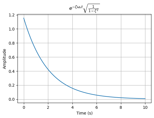
zeta = 0.5  # 阻尼比
omega_n = 1.0  # 自然频率
omega_d = omega_n * np.sqrt(1 - zeta**2)  # 阻尼频率
varphi = np.pi / 4  # 相位角

# 定义时间变量
t = np.linspace(0, 10, 1000)  # 从0到10秒，1000个点

# 计算函数值
a = np.exp(-zeta * omega_n * t) * np.sqrt(1 / (1 - zeta**2))
b = np.sin(omega_d * t + varphi)
c = np.exp(-zeta * omega_n * t) * np.sqrt(1 / (1 - zeta**2)) * np.sin(omega_d * t + varphi)

# 绘制(a)图
plt.figure(figsize=(6, 4))
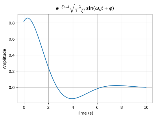
plt.plot(t, a)
plt.title(r'$e^{-\zeta\omega_{n} t}\sqrt{\frac{1}{1-\zeta^2}}$')
plt.xlabel('Time (s)')
plt.ylabel('Amplitude')
plt.grid(True)
plt.show()

# 绘制(b)图
plt.figure(figsize=(6, 4))
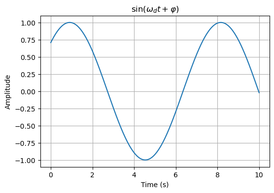
plt.plot(t, b)
plt.title(r'$\sin(\omega_{d} t+\varphi)$')
plt.xlabel('Time (s)')
plt.ylabel('Amplitude')
plt.grid(True)
plt.show()

# 绘制(c)图
plt.figure(figsize=(6, 4))
plt.plot(t, c)
plt.title(r'$e^{-\zeta\omega_{n} t}\sqrt{\frac{1}{1-\zeta^2}}\sin(\omega_{d} t+\varphi)$')
plt.xlabel('Time (s)')
plt.ylabel('Amplitude')
plt.grid(True)
plt.show()