
CT断层成像系列02——Shepp-Logan头模型的平行束投影数据仿真(Matlab|C++代码实现)
时间地点_20260123上海光源
Shepp Logan头的投影数据的数学公式推导
先上一张关键示意图, 来降低理解难度:(就叫他图2.5)
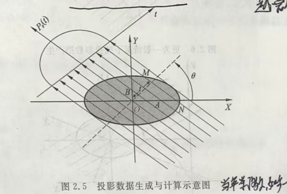
我们假设X射线面阵探测器这一行的像素序列为\(t\), 在\(t\)上的这一层切片的投影数据(灰度值)为\(P_\theta (t)\), 我们与系列01一样先从一个规规整整不旋转且椭圆中心位于中央坐标系原点\(O\)的椭圆来举例. 在CT采集的过程中, 探测器相对于坐标系是旋转的, 这一角度成为\(\theta\) 由于是同步辐射光源出光, X射线束线形状为平行束, 随着距离不会发散, 因此探测器\(t\)距离中央坐标系原点\(O\)的距离无关紧要, 离多远都不会改变投影结果, 探测器距离在讨论中被排除.
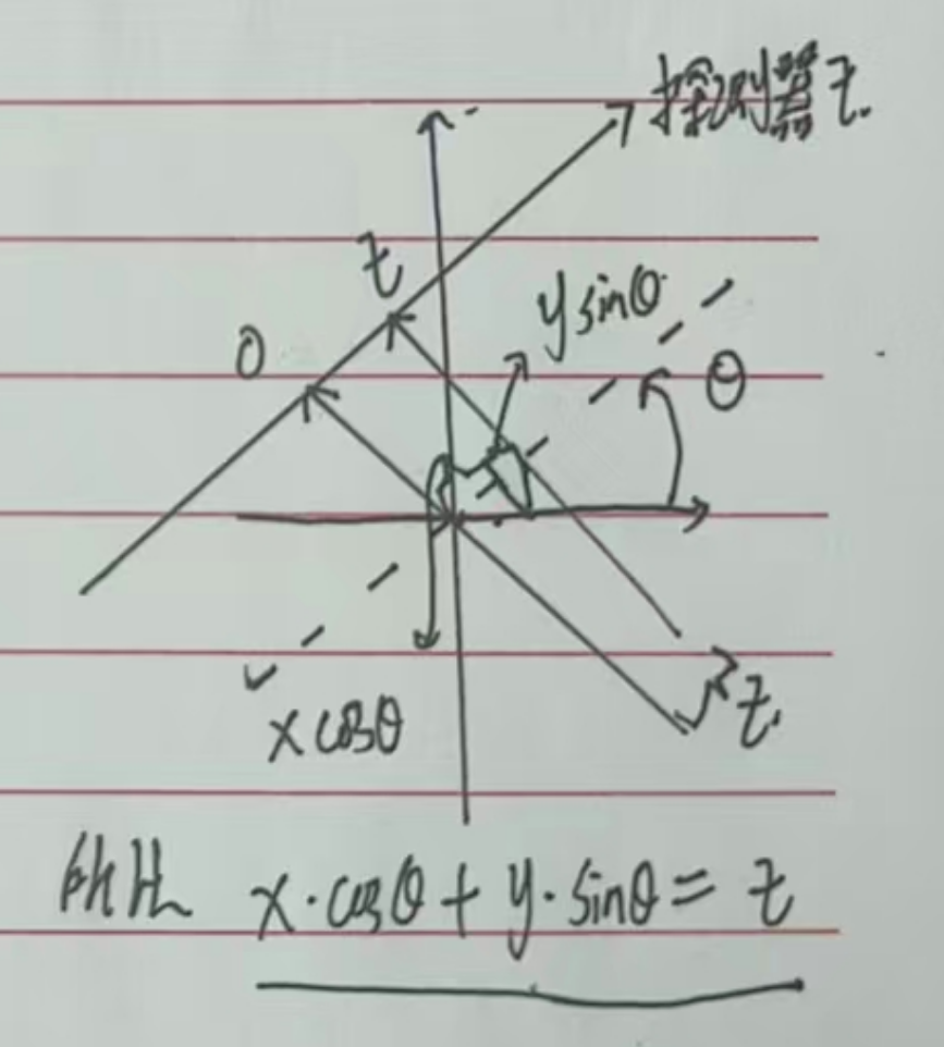
对于探测器任一像素或通道\(t\) (注意,这在算法实现上时常可以是小数), 一束射线先经过样品衰减后到达第\(t\)个像素, 这是它相对于探测器中心位置0的距离. 由我上面的草图可知, 任意打到探测器的射线都可以用\(x\)和\(y\)来表示\(t\):
对于图2.5,里的椭圆, 由系列01我们知道他的表达式为:
一束X射线MN打穿椭圆样品射线探测器的第\(t\)个像素上, 射线与椭圆相交于MN两点, 此刻t点的探测器灰度值是射线MN经过样品这一段线段的密度总衰减, 所以探测器像素\(t\) 的灰度为\(P_\theta (t)\):
\(\rho\)在SL头就是个常数, 所以求投影值就是求MN这一选段的距离. 联立公式(1)(2)(我算到昏厥也没解出来)即可求得射线经过样品的总长度MN为:
在这其中, r为;
那么MN的长度为两点相减, 为"
就像前面说的, 有了MN的长度就知道\(P_\theta (t)\)了, 这样, 投影函数\(P_\theta (t)\)的一般表达式为:
这样我们就得到了计算规整椭圆的投影数据的数学解析表达式, 下面要融合系列01里随意旋转平移的椭圆得到更泛用的解析解, 由本系列01的公式(5)可知, 一个任意旋转角度任意平移的椭圆在中央坐标系\(XOY\)的表达式为:
任意过这个椭圆的射线\(\overline{PQ}\)被椭圆吸收衰减后, 再被探测器的第\(t\)个像素通道所捕获, 该射线的表达式还是:
公式(8)(9)联立即可解得(我解不出来, 抄书了)PQ两点的坐标, 进而得到线段\(\overline{PQ}\)的长度:
在这之中:
(11)代入(10), 我们就得到了最终的Shepp-Logan头模型的投影数据的解析解, 投影函数\(P_\theta (t)\)为:
其中\(\rho、A、B、\alpha、\theta和\alpha\)分别是椭圆密度、长半轴、短半轴、旋转角和探测器旋转角。 对于S-L头模型,我们逐角度的,把每个椭圆的投影累加就得到了投影数据。 至此, 由系列01和02我把S-L头的所有知识讲完了。
Shepp Logan头的投影数据的代码实现
Matlab|直接调用Radon(拉东)函数实现SL头投影数据:
化身调包侠, 光速拿下:
clc;clear all;close all;
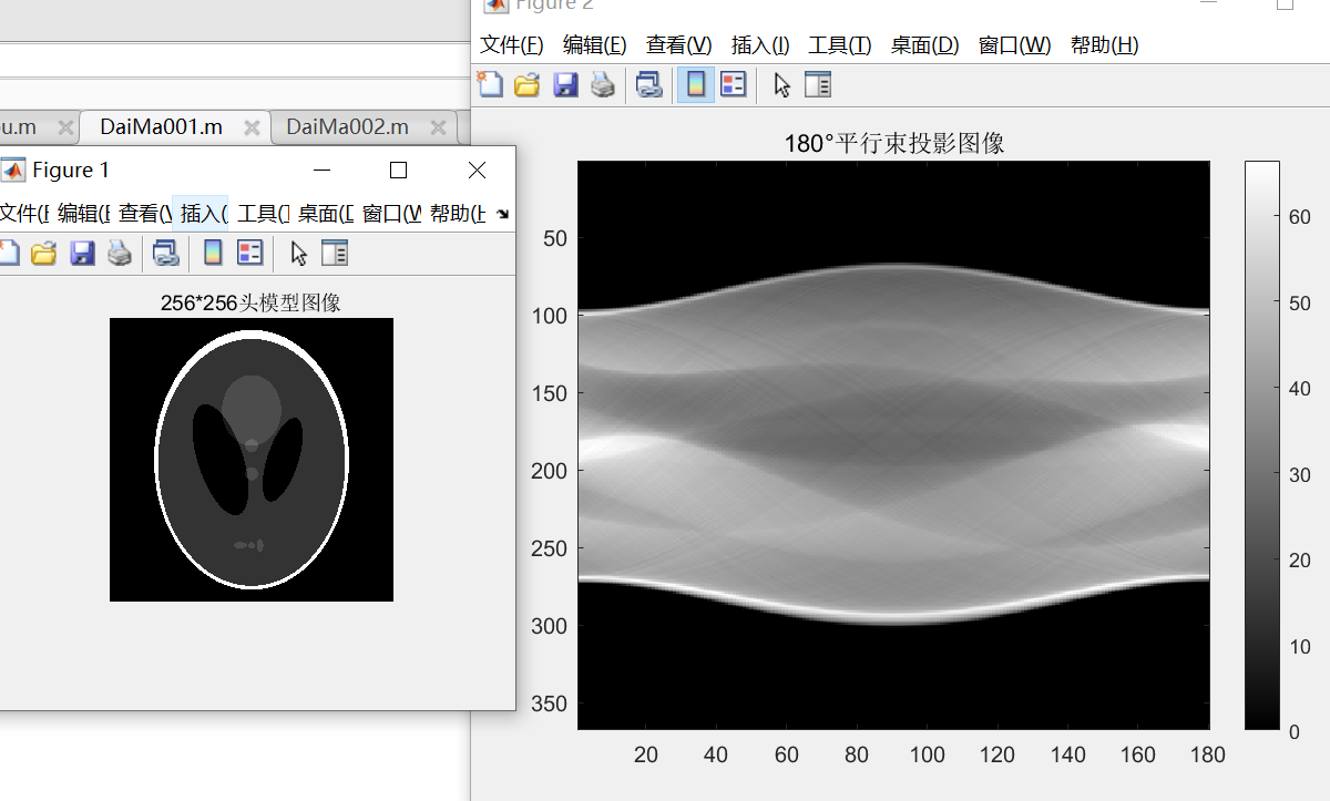
I=phantom(256);%生成256*256的Shepp Logan头模型
theta=0:179;%投影角度
P=radon(I,theta);%生成投影数据
figure;imshow(I,[]),title('256*256头模型图像');
figure;imagesc(P),colormap(gray),colorbar,title('180°平行束投影图像');
运行结果:
拉东法很泛用,啥图都能生成投影数据, 系列03讲它。
Matlab|利用数学解析法手搓SL头投影数据:
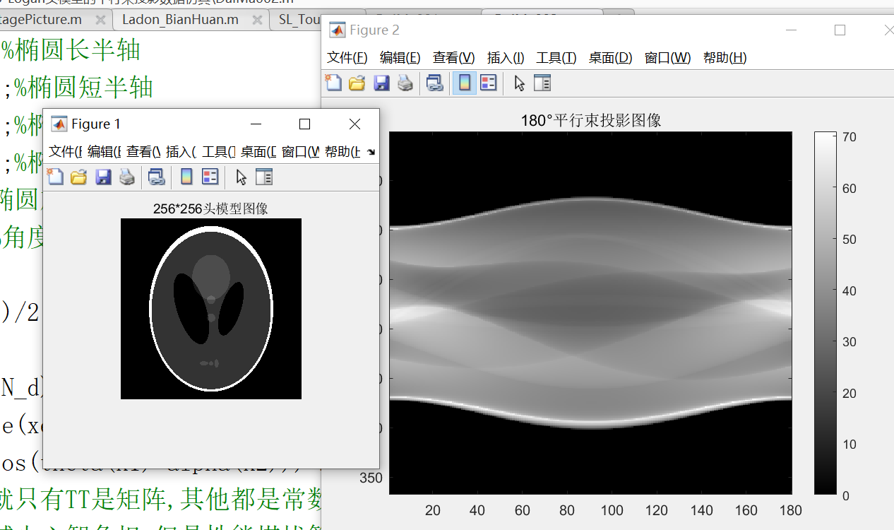
利用公式(12)手搓轮子, 数学解析的实现SL头投影数据:
    clc;clear all;close all;
    %%======仿真参数设置======%%
    N=256;%重建图像大小,探测器通道个数
    theta=0:1:179;%投影角度
    %%======产生仿真数据======%%
    I=phantom(N);	%生产Shepp_Logan头模型
    N_d=2*ceil(norm(size(I)-floor((size(I)-1)/2)-1))+3; %设定探测器通道|像素个数
    P=medfuncParallelBeamForwardProjection(theta,N,N_d); %产生投影数据
    %%======仿真结果显示======%%
    figure;imshow(I,[]),title('256*256头模型图像'); %显示原始图像
    figure;imagesc(P),colormap(gray),colorbar,title('180°平行束投影图像'); %显示投影数据


    function P=medfuncParallelBeamForwardProjection(theta,N,N_d)
    %Parallel beam forward projection function
    %-----------
    %输入参数
    %theta:探测器的旋转角度|投影角度矢量 indegrees
    %N 图像大小;N_d 探测器通道个数|一行的像素数
    %-----------
    %输出参数
    %P:投影数据矩阵(N_d*theta_num) 也就是我们平时实验得到的数据Projection
    %%========================================%%
    %椭圆绘图的六个参数 A密度|振幅 a长轴 b短轴 x0椭圆心横坐标 y0椭圆形纵坐标 α旋转角度
    shep=[
        1       .69     .92     0       0       0
        -.8     .6624   .8740   0       -.0184  0
        -.2     .1100   .3100   .22     0       -18
        -.2     .1600   .4100   -.22    0       18
        .1      .2100   .2500   0       .35     0
        .1      .0460   .0460   0       .1      0
        .1      .0460   .0460   0       -.1     0
        .1      .0460   .0230   -.08    -.605   0
        .1      .0230   .0230   0       -.606   0
        .1      .0230   .0460   .06     -.605   0
        ];
    theta_num=length(theta);
    P=zeros(N_d,theta_num);%存放投影数据
    rho=shep(:,1).';%椭圆对应密度
    %参数是百分数,乘N椭圆扩张到整个图像
    ae=0.5*N*shep(:,2)';%椭圆长半轴
    be=0.5*N*shep(:,3).';%椭圆短半轴
    xe=0.5*N*shep(:,4).';%椭圆中心x坐标
    ye=0.5*N*shep(:,5).';%椭圆中心y坐标
    alpha=shep(:,6).';%椭圆旋转角度
    alpha=alpha*pi/180;%角度变弧度
    theta=theta*pi/180;
    TT=-(N_d-1)/2:(N_d-1)/2;%探测器像素们的序列号|探测器坐标
    for k1=1:theta_num
        P_theta=zeros(1,N_d);%存放每一角度投影数据
        for k2=1:max(size(xe))
            a= (ae(k2)*cos(theta(k1)-alpha(k2)))^2+(be(k2)*sin(theta(k1)-alpha(k2)))^2;
            %整个公式串就只有TT是矩阵,其他都是常数,所以这里之后是点乘点除.Matlab可以不用逐个像素for循环,而是以矩阵直接运算
            %这样做极大减少心智负担,但是性能堪忧算的太慢,
            temp=a-(TT-xe(k2)*cos(theta(k1))-ye(k2)*sin(theta(k1))).^2;
            ind = temp>0;%根号内值需为非负
            P_theta(ind)=P_theta(ind)+rho(k2)*(2*ae(k2)*be(k2)*sqrt(temp(ind)))./a;
        end
        P(:,k1)=P_theta.';
    end

    end
运行结果如下:
C++|利用数学解析法手搓SL头投影数据:
还是那句话, Matlab也好Python也好, 这些人类友好语言都太慢太慢了, 动辄算几个小时, 这是没法落地的。据我观察, 工业届医疗届的高性能程序或者图像密集型程序都是C++写的。当然还有更底层更快的,用嵌入式或FPGA,扯远了, 附上C++实现的代码:
//  main.cpp
//  g++ main.cpp -std=c++11 `pkg-config --cflags --libs opencv4` -o slphantom

#include <opencv2/opencv.hpp>
#include <vector>
#include <cmath>

const double PI = 3.14159265358979323846;

// ---------- 1. 生成 Shepp-Logan 头模型 ----------
cv::Mat phantom(int N)
{
    // 11 个椭圆的参数:密度 长轴 短轴 中心x 中心y 旋转角(度)
    const double shep[11][6] = {
        {1.0,  0.69,  0.92,  0.0,   0.0,   0.0},
        {-0.8, 0.6624,0.874, 0.0,  -0.0184,0.0},
        {-0.2, 0.11,  0.31,  0.22,  0.0,  -18.0},
        {-0.2, 0.16,  0.41, -0.22,  0.0,   18.0},
        {0.1,  0.21,  0.25,  0.0,   0.35,  0.0},
        {0.1,  0.046, 0.046, 0.0,   0.1,   0.0},
        {0.1,  0.046, 0.046, 0.0,  -0.1,   0.0},
        {0.1,  0.046, 0.023,-0.08, -0.605, 0.0},
        {0.1,  0.023, 0.023, 0.0,  -0.606, 0.0},
        {0.1,  0.023, 0.046, 0.06, -0.605, 0.0}
    };

    cv::Mat img = cv::Mat::zeros(N, N, CV_64F);
    double cx = (N - 1) * 0.5, cy = cx;

    for (int y = 0; y < N; ++y)
    {
        double yy = y - cy;
        for (int x = 0; x < N; ++x)
        {
            double xx = x - cx;
            double val = 0.0;
            for (int k = 0; k < 10; ++k)
            {
                double rho = shep[k][0];
                double a = shep[k][1] * N * 0.5;
                double b = shep[k][2] * N * 0.5;
                double x0 = shep[k][3] * N * 0.5;
                double y0 = shep[k][4] * N * 0.5;
                double alpha = shep[k][5] * PI / 180.0;

                double x1 = (xx - x0) * cos(alpha) + (yy - y0) * sin(alpha);
                double y1 = -(xx - x0) * sin(alpha) + (yy - y0) * cos(alpha);
                double r2 = (x1 * x1) / (a * a) + (y1 * y1) / (b * b);
                if (r2 <= 1.0) val += rho;
            }
            img.at<double>(y, x) = val;
        }
    }
    cv::Mat out;
    cv::normalize(img, out, 0, 255, cv::NORM_MINMAX, CV_8U);
    return out;
}

// ---------- 2. 平行束前向投影 ----------
cv::Mat medfuncParallelBeamForwardProjection(const std::vector<double>& thetaDeg,
    int N, int N_d)
{
    // 同样 10 个椭圆参数(只取前 10 个,和 MATLAB 一致)
    const double shep[10][6] = {
        {1.0,  0.69,  0.92,  0.0,   0.0,   0.0},
        {-0.8, 0.6624,0.874, 0.0,  -0.0184,0.0},
        {-0.2, 0.11,  0.31,  0.22,  0.0,  -18.0},
        {-0.2, 0.16,  0.41, -0.22,  0.0,   18.0},
        {0.1,  0.21,  0.25,  0.0,   0.35,  0.0},
        {0.1,  0.046, 0.046, 0.0,   0.1,   0.0},
        {0.1,  0.046, 0.046, 0.0,  -0.1,   0.0},
        {0.1,  0.046, 0.023,-0.08, -0.605, 0.0},
        {0.1,  0.023, 0.023, 0.0,  -0.606, 0.0},
        {0.1,  0.023, 0.046, 0.06, -0.605, 0.0}
    };

    int nAng = thetaDeg.size();
    cv::Mat P = cv::Mat::zeros(N_d, nAng, CV_64F);   // 投影矩阵

    // 把椭圆参数一次性换算到像素坐标
    std::vector<double> rho(10), ae(10), be(10), xe(10), ye(10), alpha(10);
    for (int k = 0; k < 10; ++k)
    {
        rho[k] = shep[k][0];
        ae[k] = shep[k][1] * N * 0.5;
        be[k] = shep[k][2] * N * 0.5;
        xe[k] = shep[k][3] * N * 0.5;
        ye[k] = shep[k][4] * N * 0.5;
        alpha[k] = shep[k][5] * PI / 180.0;
    }

    // 探测器坐标 [-range ... +range]
    std::vector<double> TT(N_d);
    for (int i = 0; i < N_d; ++i) TT[i] = i - (N_d - 1) * 0.5;

    for (int k1 = 0; k1 < nAng; ++k1)
    {
        double th = thetaDeg[k1] * PI / 180.0;
        std::vector<double> P_theta(N_d, 0.0);

        for (int k2 = 0; k2 < 10; ++k2)
        {
            double ca = cos(th - alpha[k2]);
            double sa = sin(th - alpha[k2]);
            double a = ae[k2] * ae[k2] * ca * ca + be[k2] * be[k2] * sa * sa;

            double xc = xe[k2] * cos(th) + ye[k2] * sin(th);

            for (int i = 0; i < N_d; ++i)
            {
                double t = TT[i] - xc;
                double tmp = a - t * t;
                if (tmp > 0)
                {
                    double len = 2.0 * ae[k2] * be[k2] * sqrt(tmp) / a;
                    P_theta[i] += rho[k2] * len;
                }
            }
        }
        // 写回列向量
        for (int i = 0; i < N_d; ++i)
            P.at<double>(i, k1) = P_theta[i];
    }
    return P;
}

// ---------- 3. 主函数 ----------
int main()
{
    const int N = 256;
    const int N_d = 2 * static_cast<int>(
        std::ceil(std::sqrt(2.0) * (N - 1) * 0.5)) + 3;

    std::vector<double> thetaDeg;
    for (int i = 0; i < 180; ++i) thetaDeg.push_back(i);   // 0~179°

    // 1. 生成头模型
    cv::Mat I = phantom(N);
    // 2. 前向投影
    cv::Mat P = medfuncParallelBeamForwardProjection(thetaDeg, N, N_d);

    // 3. 显示
    cv::imshow("256×256 Shepp-Logan", I);            // 缩放到 0~1 方便显示
    cv::Mat P_show;
    cv::normalize(P, P_show, 0, 1, cv::NORM_MINMAX);
    cv::imshow("180° Parallel-beam sinogram", P_show);
    cv::waitKey(0);

    // 4. 可选:写盘
    //cv::imwrite("phantom.png", I * 255);
    // cv::imwrite("sinogram.png", P_show * 255);
    return 0;
}
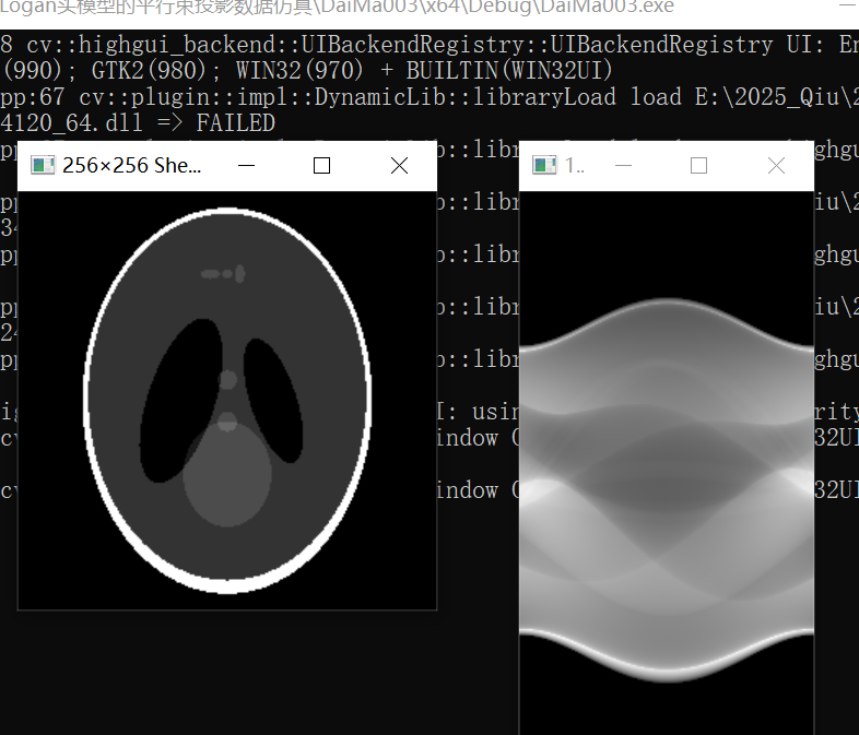
运行结果如下:
结束, 系列03介绍更通用的投影数据获得方法——拉东函数正向投影, 进而还能引出拉东反向投影,也就是CT重建算法FBP了

 浙公网安备 33010602011771号