第一次作业：深度学习基础

# 1.视频学习总结

1.1绪论

什么是人工智能？

人工智能是使一个机器像人一样进行感知、认知、决策、执行的人工程序或系统。

什么是图灵测试？

图灵测试是指测试者与被测试者（一个人和一台机器）隔开的情况下，通过一些装置（如键盘）向被测试者随意提问，进行多次测试后，如果机器让平均每个参与者做出超过30%的误判，那么这台机器就通过了测试，并被认为具有人类智能。

人工智能发展阶段：萌芽期，启动期，消沉期，突破期，发展期，高速发展期。

人工智能三个层面：计算智能、感知智能、认知智能。

实现人工智能有两条脉络：专家系统与机器学习

专家系统：根据专家定义的知识和经验，进行推理和判断，从而模拟人类专家的决策过程来解决问题。

机器学习：是用数据或以往的经验，以此优化计算机程序的性能标准。

机器学习三要素：模型、策略、算法。

模型：对要学习问题映射的假设（问题模型，确定假设空间）

策略：从假设空间中学习、选择最优模型的准则（确定目标函数）

算法：根据目标函数求解最优模型的具体计算方法（求解模型参数）

模型分类：数据标记（监督学习、无监督学习、半监督学习、强化学习）、数据分布（参数模型，非参数模型）、建模对象（判别模型、生成模型）

深度学习三个助推剂：数据、算法、计算力

深度学习的不能：算法输出不稳定，容易被攻击；模型复杂度高，难以纠错和调试；模型层级复合程度高，参数不透明；端到端训练方式对数据依赖性强，模型增量性差；专注直观感知类问题，对开放性推理问题无能为力；人类知识无法有效引入进行监督，机器偏见难以避免。

1.2神经网络基础

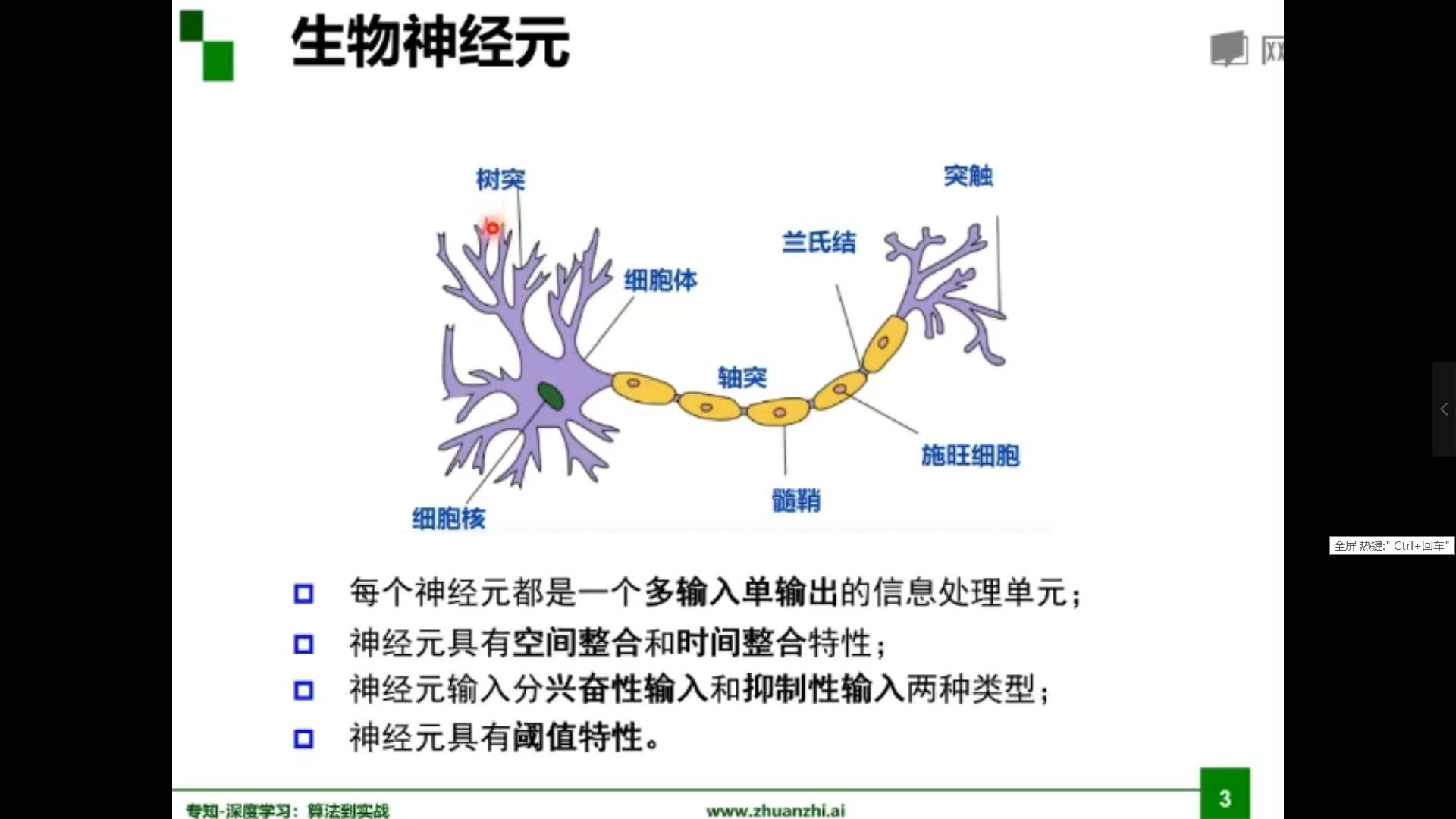
生物神经元

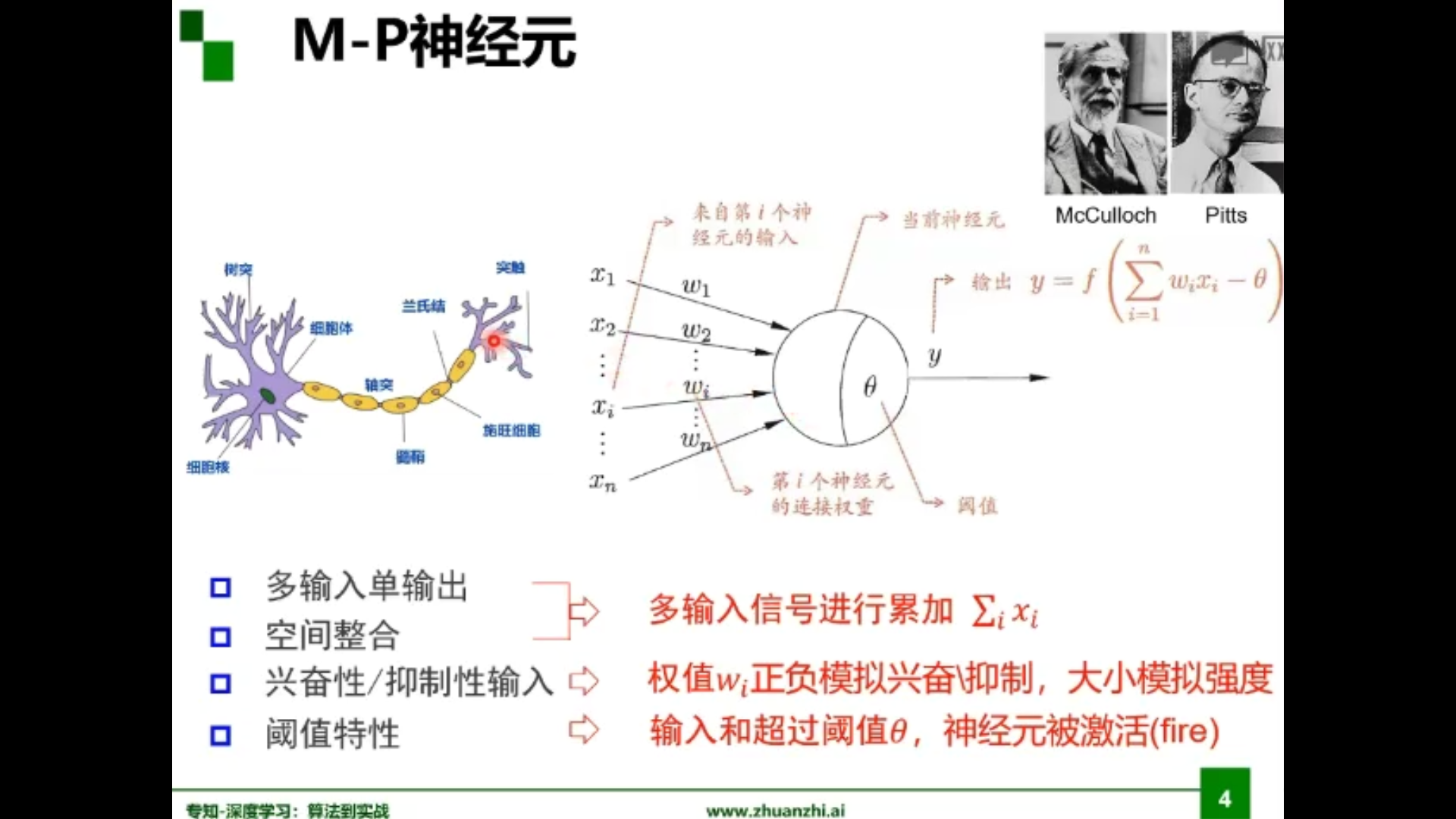
M-P神经元

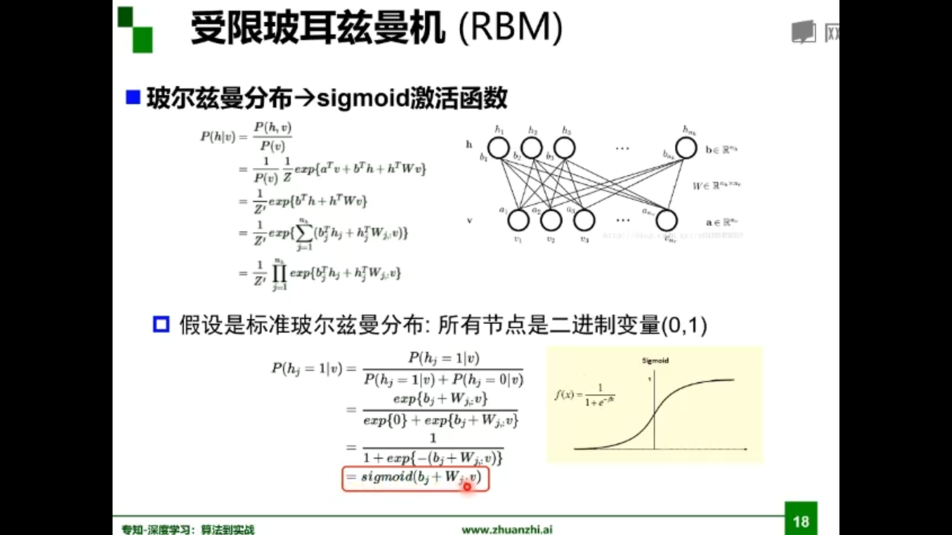
为什么需要激活函数？

神经网络中激活函数的主要作用是提供网络的非线性建模能力，如不特别说明，激活函数一般而言是非线性函数。假设一个示例神经网络中仅包含线性卷积和全连接运算，那么该网络仅能够表达线性映射，即便增加网络的深度也依旧还是线性映射，难以有效建模实际环境中非线性分布的数据。加入（非线性）激活函数之后，深度神经网络才具备了分层的非线性映射学习能力。

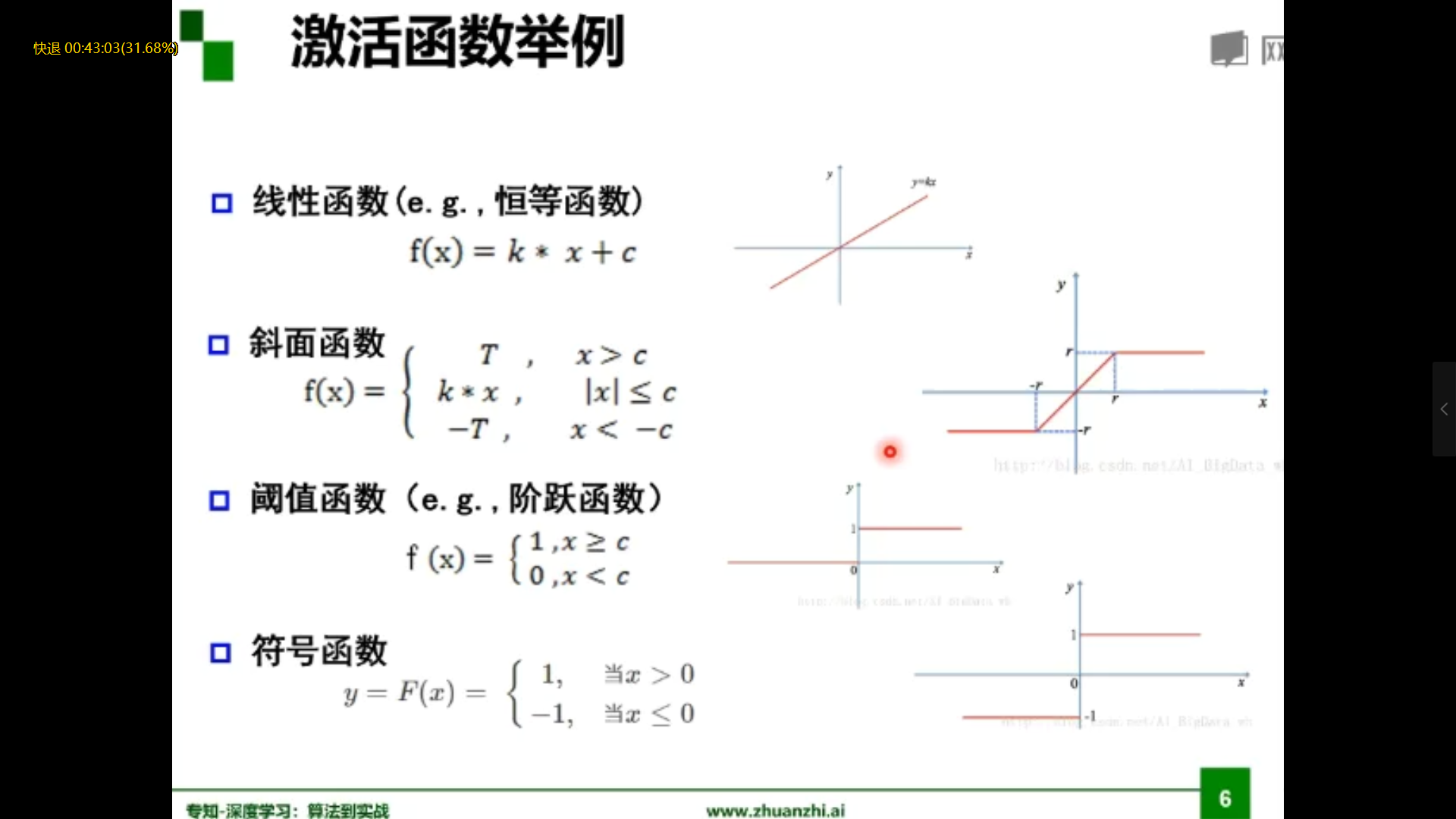
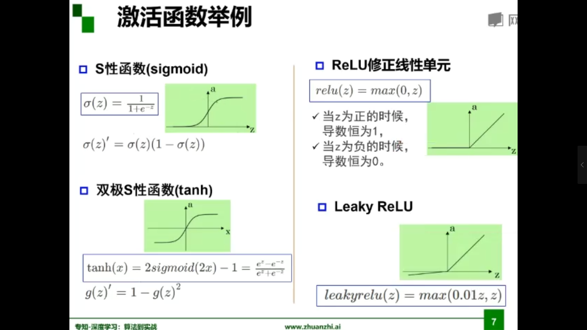
激活函数举例

单层感知器

是首个可以学习的人工神经网络

可以实现简单的逻辑与、或、非操作，解决不了异或问题

多层感知器

通过加隐层将一个非线性问题转化为线性问题

万有逼近定理

如果一个隐层包含足够多的神经元，三层前馈网络（输入-隐层-输出）能任意精度逼近任意预定的连续函数。

双层感知器逼近非连续函数。当隐层足够宽时，双隐层感知器可以逼近任意非连续函数，可解决任何复杂的分类问题。

为什么线性分类任务组合后可以解决非线性分类任务？

经过隐层变换后相当于进行了空间变换，将非线性分类任务转换为线性问题。

神经网络每一层作用

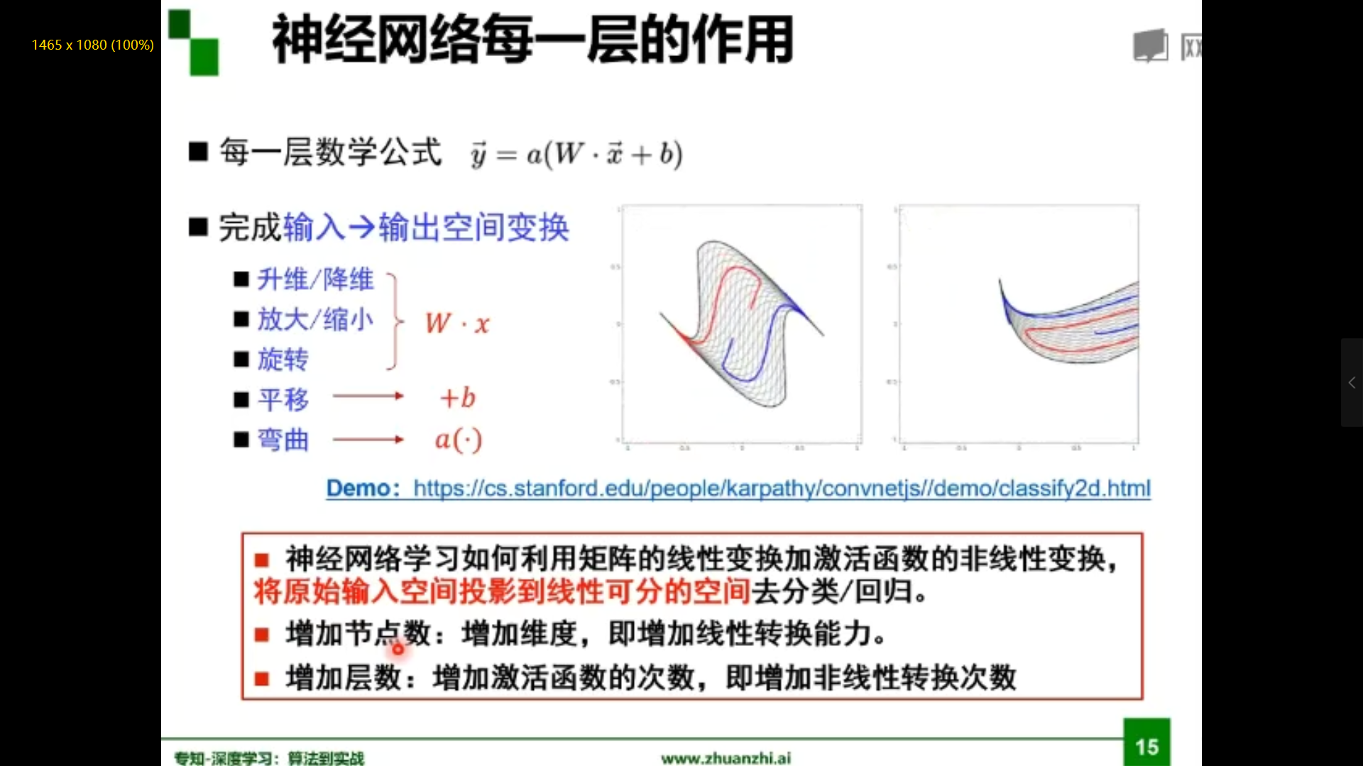
更深 or 更宽

在神经元总数相当的情况下，增加网络深度可比增加宽度带来更强的网络表示能力：产生更多地线性区域。深度的贡献是指数增长的，而宽度的贡献是线性的。

误差反向传播

利用误差更新网络参数，利用梯度完成，是一种复合函数的链式求导。

梯度与梯度下降

梯度：某一函数在该点处的方向导数沿着该方向取得最大值

梯度下降：是一种无约束优化方法，参数沿着负梯度方向更新可以使函数值下降，可能无法找到全局的极值点，而是找到局部极值点。

梯度消失问题

误差无法传播，参数过小，只更新了最后一层参数，前面的参数没有更新

梯度消失问题怎么解决？

逐层预训练，更换激活函数，辅助损失函数，逐层的尺度归一。

逐层预训练（layer-wise pre-training）

每次训练一个三层的网络，将训练结果迭代到后面。收敛好，次数少。保证从初始就不会太差。

受限玻尔兹曼机与自编码器

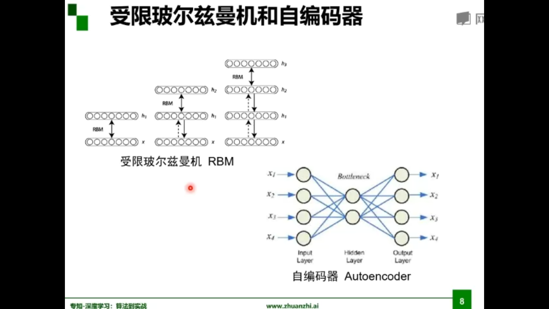
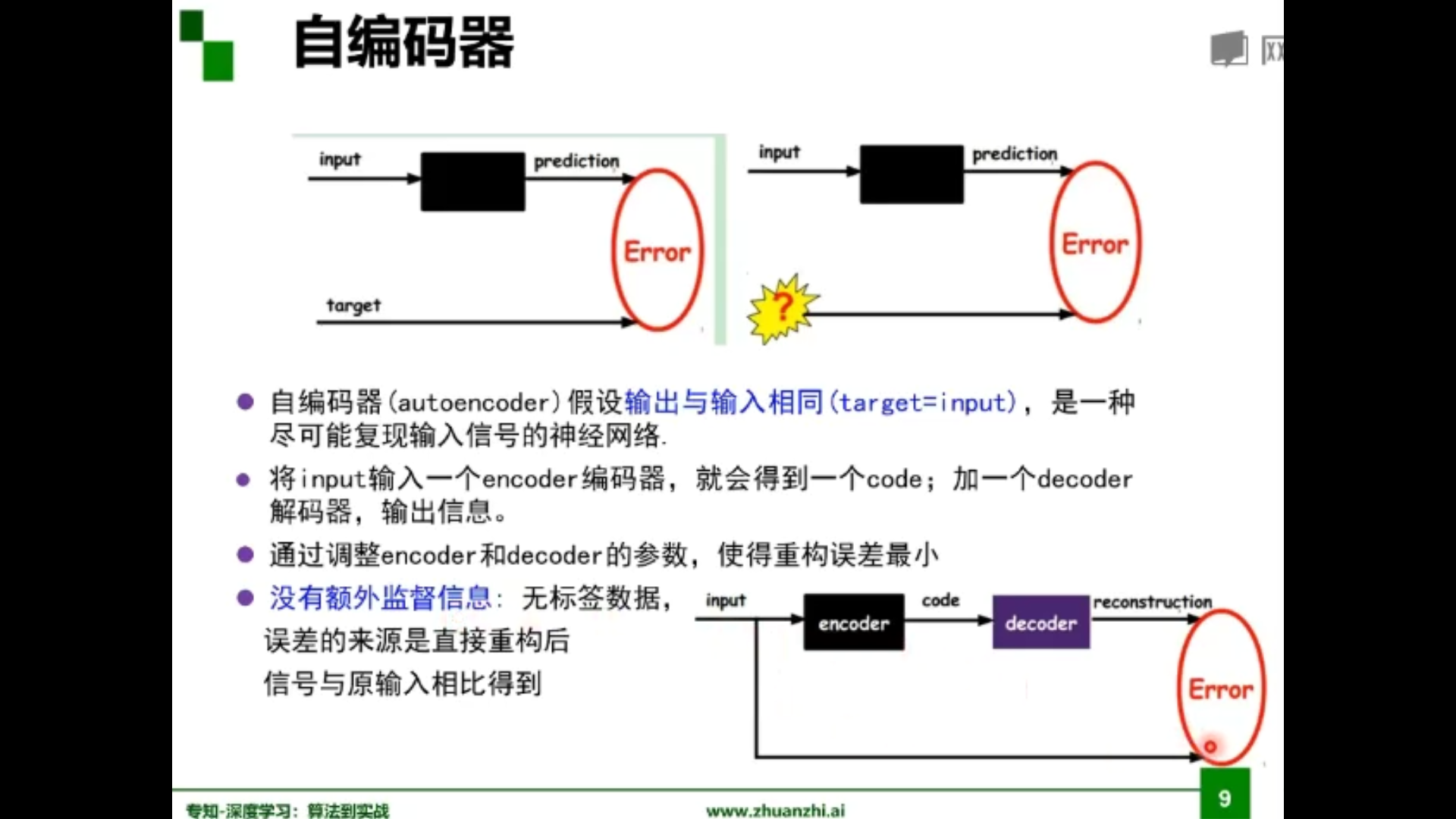
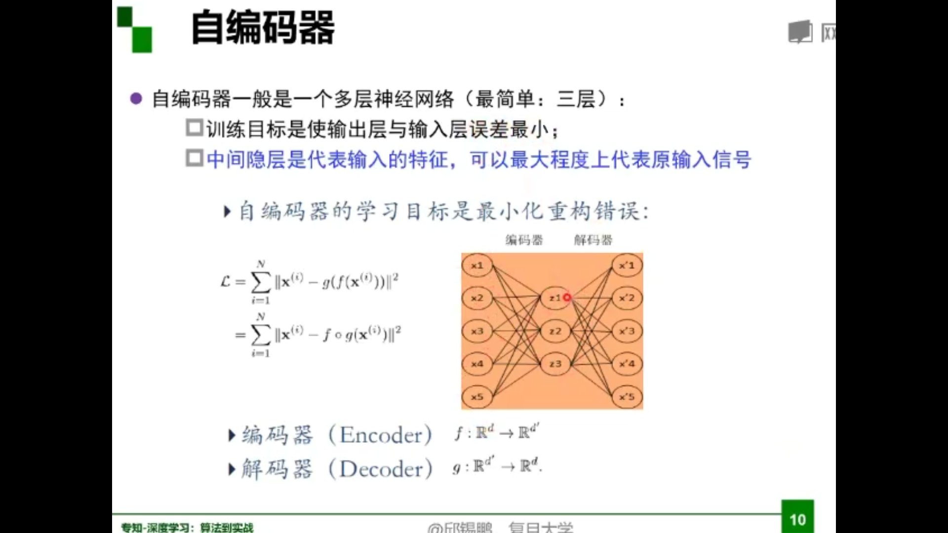
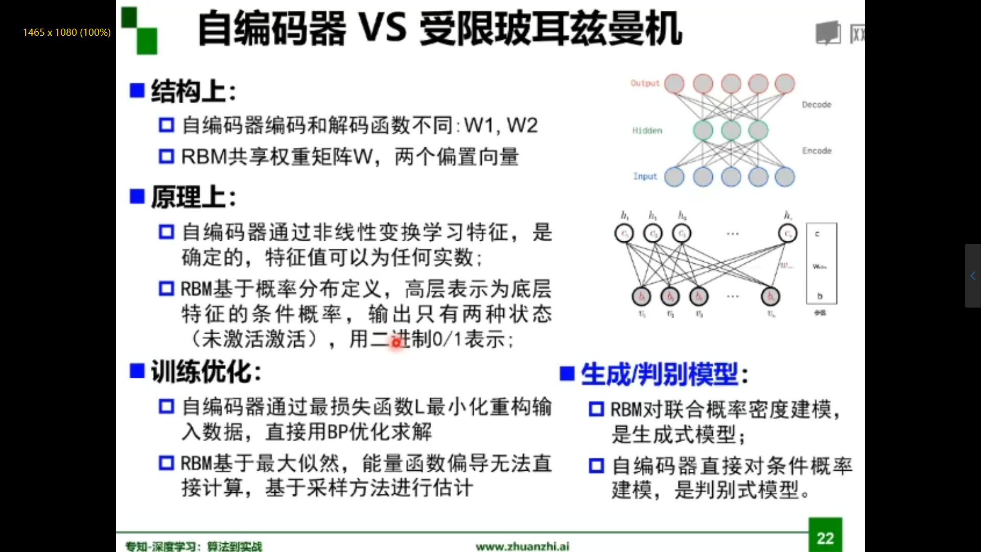
自编码器

堆叠自编码器

将多个自编码器得到的隐层串联；将所有层预训练完成后，进行基于监督学习的全网络微调。先编码再解码。是一个框架。

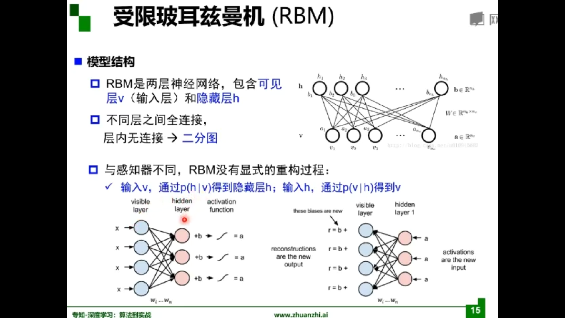
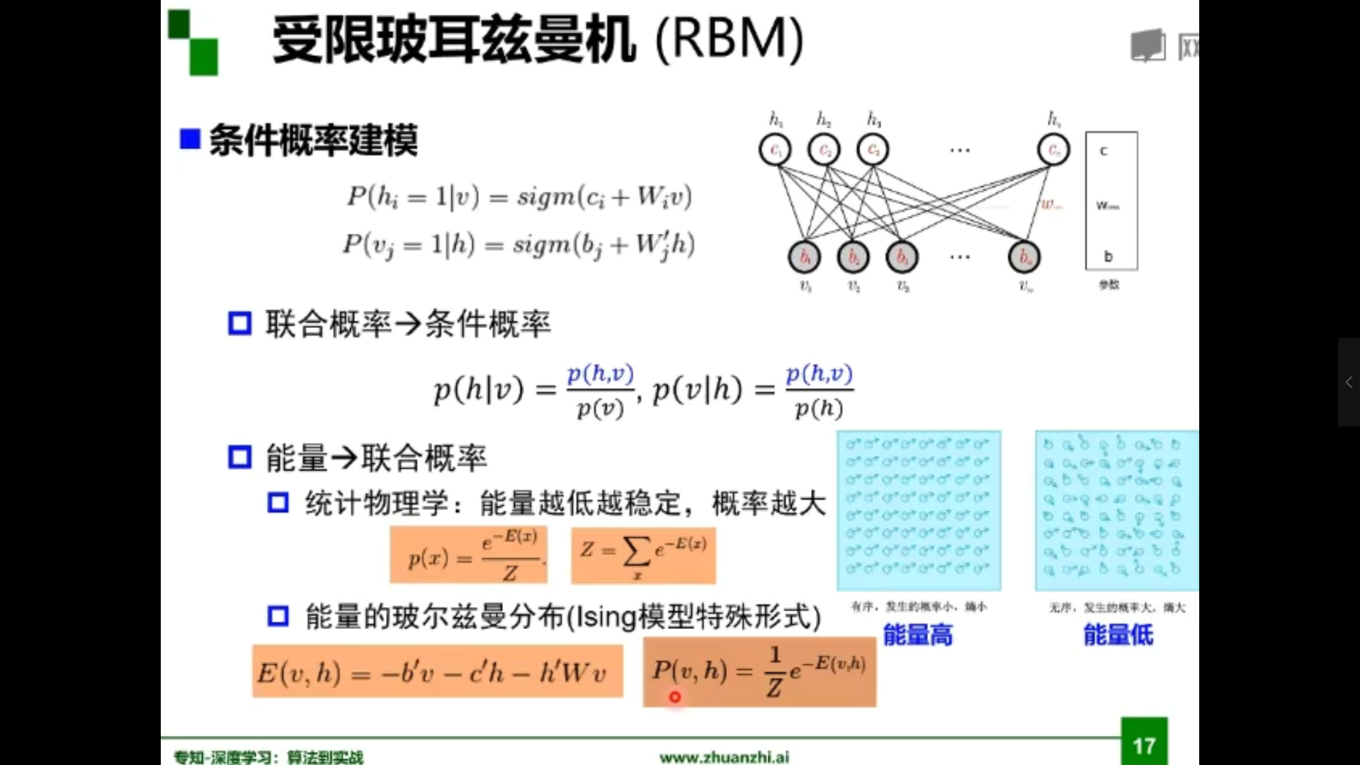
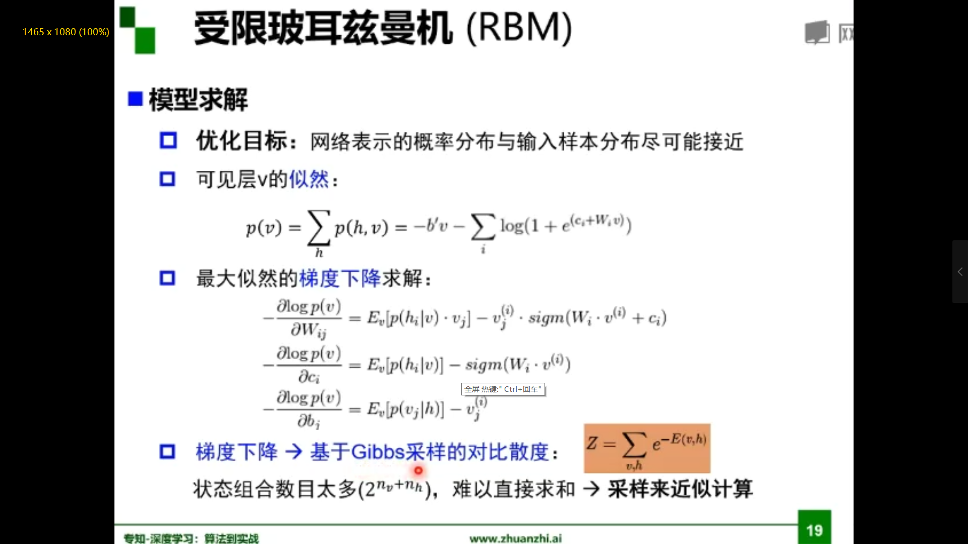
受限玻尔兹曼机

自编码器与受限玻尔兹曼机比较

2.代码练习

2.1 图像处理基本练习

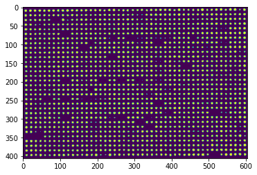
1.下载并显示图像

!wget https://raw.githubusercontent.com/summitgao/ImageGallery/master/yeast_colony_array.jpg

import matplotlib
import numpy as np
import matplotlib.pyplot as plt

import skimage
from skimage import data
from skimage import io

colony = io.imread('yeast_colony_array.jpg')
print(type(colony))
print(colony.shape)

<class 'numpy.ndarray'>
(406, 604, 3)

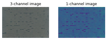
# Plot all channels of a real image
plt.subplot(121)
plt.imshow(colony[:,:,:])
plt.title('3-channel image')
plt.axis('off')

# Plot one channel only
plt.subplot(122)
plt.imshow(colony[:,:,0])
plt.title('1-channel image')
plt.axis('off');

2.读取并改变图像像素值

# Get the pixel value at row 10, column 10 on the 10th row and 20th column
camera = data.camera()
print(camera[10, 20])

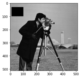
# Set a region to black
camera[30:100, 10:100] = 0
plt.imshow(camera, 'gray')

153
<matplotlib.image.AxesImage at 0x7fd4fc859198>

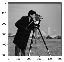
# Set the first ten lines to black
camera = data.camera()
camera[:10] = 0
plt.imshow(camera, 'gray')

<matplotlib.image.AxesImage at 0x7fd4fc849470>

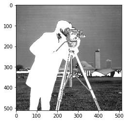
# Set to "white" (255) pixels where mask is True
camera = data.camera()
mask = camera < 80
camera[mask] = 255
plt.imshow(camera, 'gray')

<matplotlib.image.AxesImage at 0x7fd4fc7fdbe0>

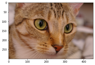
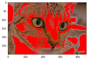
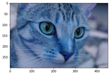
# Change the color for real images
cat = data.chelsea()
plt.imshow(cat)

<matplotlib.image.AxesImage at 0x7fd4fe6107b8>

# Set brighter pixels to red
red_cat = cat.copy()
reddish = cat[:, :, 0] > 160
red_cat[reddish] = [255, 0, 0]
plt.imshow(red_cat)

<matplotlib.image.AxesImage at 0x7fd4fc7cd320>

# Change RGB color to BGR for openCV
BGR_cat = cat[:, :, ::-1]
plt.imshow(BGR_cat)

<matplotlib.image.AxesImage at 0x7fd4fc726a90>

3.转换图像数据类型

from skimage import img_as_float, img_as_ubyte
float_cat = img_as_float(cat)
uint_cat = img_as_ubyte(float_cat)

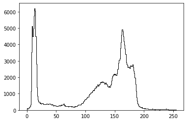
4.显示直方图

img = data.camera()
plt.hist(img.ravel(), bins=256, histtype='step', color='black');

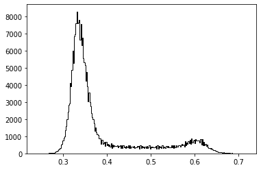
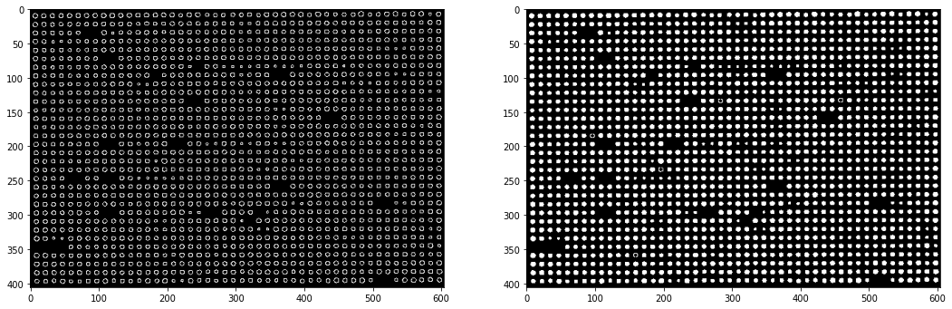
5.图像分割

# Use colony image for segmentation
colony = io.imread('yeast_colony_array.jpg')

# Plot histogram
img = skimage.color.rgb2gray(colony)
plt.hist(img.ravel(), bins=256, histtype='step', color='black');

# Use thresholding
plt.imshow(img>0.5)

<matplotlib.image.AxesImage at 0x7fd4fc5d84a8>

6.Canny算子用于边缘检测

from skimage.feature import canny
from scipy import ndimage as ndi
img_edges = canny(img)
img_filled = ndi.binary_fill_holes(img_edges)

# Plot
plt.figure(figsize=(18, 12))
plt.subplot(121)
plt.imshow(img_edges, 'gray')
plt.subplot(122)
plt.imshow(img_filled, 'gray')

<matplotlib.image.AxesImage at 0x7fd4ee361160>

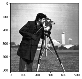
7.改变图像的对比度

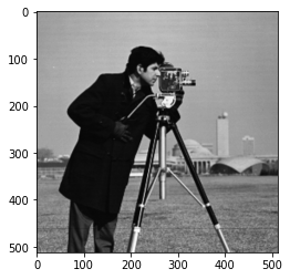
# Load an example image
img = data.camera()
plt.imshow(img, 'gray')

<matplotlib.image.AxesImage at 0x7fd4ee2ac400>

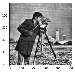
from skimage import exposure
# Contrast stretching
p2, p98 = np.percentile(img, (2, 98))
img_rescale = exposure.rescale_intensity(img, in_range=(p2, p98))
plt.imshow(img_rescale, 'gray')

<matplotlib.image.AxesImage at 0x7fd4ee286940>

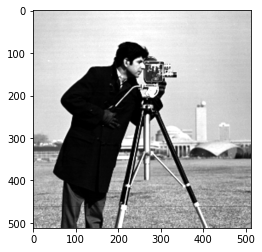
# Equalization
img_eq = exposure.equalize_hist(img)
plt.imshow(img_eq, 'gray')

<matplotlib.image.AxesImage at 0x7fd4ee1ed6d8>

# Adaptive Equalization
img_adapteq = exposure.equalize_adapthist(img, clip_limit=0.03)
plt.imshow(img_adapteq, 'gray')

<matplotlib.image.AxesImage at 0x7fd4ee1ce860>

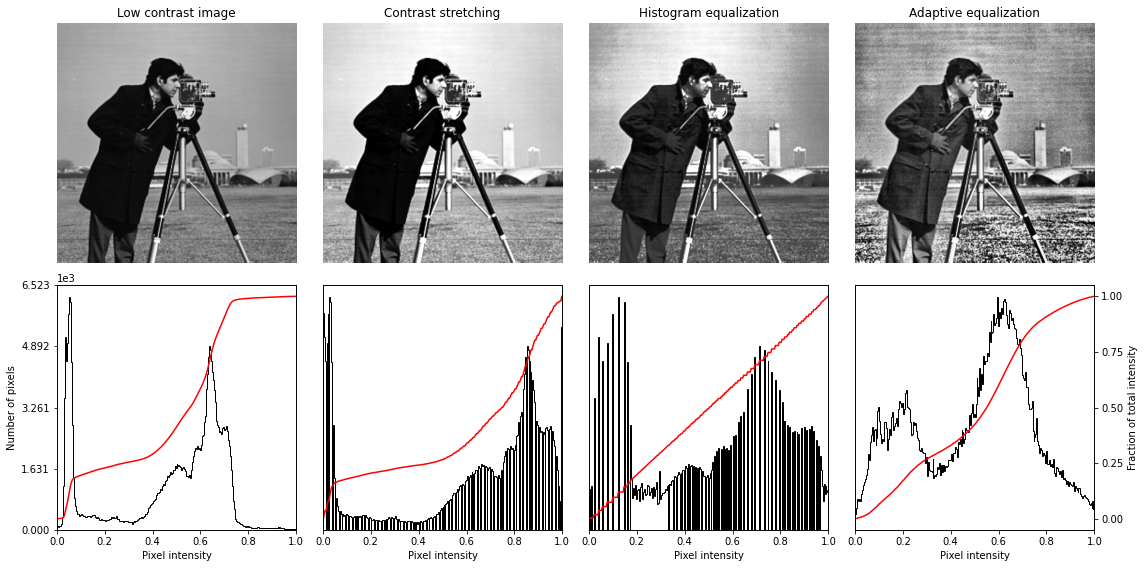
# Display results
def plot_img_and_hist(img, axes, bins=256):
    """Plot an image along with its histogram and cumulative histogram.

    """
    img = img_as_float(img)
    ax_img, ax_hist = axes
    ax_cdf = ax_hist.twinx()

    # Display image
    ax_img.imshow(img, cmap=plt.cm.gray)
    ax_img.set_axis_off()
    ax_img.set_adjustable('box')

    # Display histogram
    ax_hist.hist(img.ravel(), bins=bins, histtype='step', color='black')
    ax_hist.ticklabel_format(axis='y', style='scientific', scilimits=(0, 0))
    ax_hist.set_xlabel('Pixel intensity')
    ax_hist.set_xlim(0, 1)
    ax_hist.set_yticks([])

    # Display cumulative distribution
    img_cdf, bins = exposure.cumulative_distribution(img, bins)
    ax_cdf.plot(bins, img_cdf, 'r')
    ax_cdf.set_yticks([])

    return ax_img, ax_hist, ax_cdf

fig = plt.figure(figsize=(16, 8))
axes = np.zeros((2, 4), dtype=np.object)
axes[0, 0] = fig.add_subplot(2, 4, 1)
for i in range(1, 4):
    axes[0, i] = fig.add_subplot(2, 4, 1+i, sharex=axes[0,0], sharey=axes[0,0])
for i in range(0, 4):
    axes[1, i] = fig.add_subplot(2, 4, 5+i)

ax_img, ax_hist, ax_cdf = plot_img_and_hist(img, axes[:, 0])
ax_img.set_title('Low contrast image')

y_min, y_max = ax_hist.get_ylim()
ax_hist.set_ylabel('Number of pixels')
ax_hist.set_yticks(np.linspace(0, y_max, 5))

ax_img, ax_hist, ax_cdf = plot_img_and_hist(img_rescale, axes[:, 1])
ax_img.set_title('Contrast stretching')

ax_img, ax_hist, ax_cdf = plot_img_and_hist(img_eq, axes[:, 2])
ax_img.set_title('Histogram equalization')

ax_img, ax_hist, ax_cdf = plot_img_and_hist(img_adapteq, axes[:, 3])
ax_img.set_title('Adaptive equalization')

ax_cdf.set_ylabel('Fraction of total intensity')
ax_cdf.set_yticks(np.linspace(0, 1, 5))

fig.tight_layout()
plt.show()

2.2Pytorch基础练习

什么是Pytorch？

PyTorch是一个Python库，主要提供了以下两个高级功能：GPU加速的张量计算功能；构建在反向自动求导系统上的深度神经网络功能。

优点：Python库、符合直觉

PyTorch基础概念

怎么定义数据：张量类 torch.Tensor 任意类型的数据

怎么定义数据操作：函数类 torch.autograd.Function

凡是用torch进行的操作都是Function：基本运算、布尔运算、线性运算等。

Tensor三个重要组成：data（存数据）、grad（存梯度）、grad_fn（用来指向创造自己的Function）

计算图：计算过程的总结

PyTorch：动态图

PyTorch里没有一个显式的graph的定义，计算步骤，存在Tensor的grad_fn里沿着Tensor的grad_fn往后走，就是反向传播

1.定义数据

#一个数
import torch
x = torch.tensor(125)
print(x)

tensor(125)

#一维数组
x = torch.tensor([1,2,3])
print(x)

tensor([1, 2, 3])

#二维数组
x = torch.ones(2,3)
print(x)

tensor([[1., 1., 1.],
        [1., 1., 1.]])

#任意维数组
x = torch.ones(3,3,3)
print(x)

tensor([[[1., 1., 1.],
         [1., 1., 1.],
         [1., 1., 1.]],

        [[1., 1., 1.],
         [1., 1., 1.],
         [1., 1., 1.]],

        [[1., 1., 1.],
         [1., 1., 1.],
         [1., 1., 1.]]])

#创建空张量
x = torch.empty(3,3)
print(x)

tensor([[3.5473e-35, 0.0000e+00, 3.3631e-44],
        [0.0000e+00,        nan, 0.0000e+00],
        [1.1578e+27, 1.1362e+30, 7.1547e+22]])

#创建一个随机初始化的张量
x = torch.rand(3,3)
print(x)

tensor([[0.3742, 0.3550, 0.0759],
        [0.9095, 0.4695, 0.4756],
        [0.6537, 0.8004, 0.8611]])

#创建一个全为0的张量，并将数据类型设为long
x = torch.zeros(3,3,dtype=torch.long)
print(x)

tensor([[0, 0, 0],
        [0, 0, 0],
        [0, 0, 0]])

#基于现有的tensor，创建一个新的tensor，使新的tensor可以继承原有tensor的属性
y = x.new_ones(3,3)
print(y)

tensor([[1, 1, 1],
        [1, 1, 1],
        [1, 1, 1]])

#继承原来tensor的大小，重新定义了数据类型
z = torch.randn_like(x,dtype = torch.float)
print(z)

tensor([[-0.7898,  1.3768, -0.1248],
        [ 1.3547,  1.4419,  0.3841],
        [ 0.6716,  0.3616,  0.0647]])

2.定义操作

#创建一个2x4的tensor，用Tensor创建出来的是浮点数，用tensor创建出来的是长整型
m = torch.tensor([[2,5,3,7],[4,2,1,9]])
print(m.size(0),m.size(1),m.size(),sep = '-')

2-4-torch.Size([2, 4])

#返回m中元素的数量
print(m.numel())

8

#返回m中的元素，利用下标标记元素
print(m[0][2])
print(m[:,1])
print(m[0,:])

tensor(3)
tensor([5, 2])
tensor([2, 5, 3, 7])

#点乘
v = torch.arange(1, 5)
m @ v
m[[0], :] @ v

tensor([49, 47])
tensor([49])

#加法
m + torch.rand(2, 4)

tensor([[2.0331, 5.2091, 3.8029, 7.1205],
        [4.2729, 2.8246, 1.6806, 9.4089]])

#转置
print(m.t())
print(m.transpose(0,1))

tensor([[2, 4],
        [5, 2],
        [3, 1],
        [7, 9]])
tensor([[2, 4],
        [5, 2],
        [3, 1],
        [7, 9]])

#返回3到8之间等距的20个数
torch.linspace(3,8,20)

tensor([3.0000, 3.2632, 3.5263, 3.7895, 4.0526, 4.3158, 4.5789, 4.8421, 5.1053,
        5.3684, 5.6316, 5.8947, 6.1579, 6.4211, 6.6842, 6.9474, 7.2105, 7.4737,
        7.7368, 8.0000])

#转换数据类型并显示
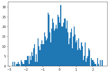
from matplotlib import pyplot as plt
plt.hist(torch.randn(1000).numpy(),100);

#数组拼接
a = torch.Tensor([[1,2,3,4]])
b = torch.Tensor([[5,6,7,8]])
print(torch.cat((a,b),0))#在0方向即在Y方向上拼接
print(torch.cat((a,b),1))#在1方向即在X方向上拼接

tensor([[1., 2., 3., 4.],
        [5., 6., 7., 8.]])
tensor([[1., 2., 3., 4., 5., 6., 7., 8.]])

2.3 螺旋数据分类

#数据初始化
import random
import torch
from torch import nn, optim
import math
from IPython import display
from plot_lib import plot_data, plot_model, set_default

# 因为colab是支持GPU的，torch 将在 GPU 上运行
device = torch.device("cuda:0" if torch.cuda.is_available() else "cpu")

# 初始化随机数种子。神经网络的参数都是随机初始化的，
# 不同的初始化参数往往会导致不同的结果，当得到比较好的结果时我们通常希望这个结果是可以复现的，
# 因此，在pytorch中，通过设置随机数种子也可以达到这个目的
seed = 12345
random.seed(seed)
torch.manual_seed(seed)

N = 1000  # 每类样本的数量
D = 2  # 每个样本的特征维度
C = 3  # 样本的类别
H = 100  # 神经网络里隐层单元的数量
X = torch.zeros(N * C, D).to(device)
Y = torch.zeros(N * C, dtype=torch.long).to(device)
for c in range(C):
    index = 0
    t = torch.linspace(0, 1, N) # 在[0，1]间均匀的取10000个数，赋给t
    # 下面的代码不用理解太多，总之是根据公式计算出三类样本（可以构成螺旋形）
    # torch.randn(N) 是得到 N 个均值为0，方差为 1 的一组随机数，注意要和 rand 区分开
    inner_var = torch.linspace( (2*math.pi/C)*c, (2*math.pi/C)*(2+c), N) + torch.randn(N) * 0.2
    
    # 每个样本的(x,y)坐标都保存在 X 里
    # Y 里存储的是样本的类别，分别为 [0, 1, 2]
    for ix in range(N * c, N * (c + 1)):
        X[ix] = t[index] * torch.FloatTensor((math.sin(inner_var[index]), math.cos(inner_var[index])))
        Y[ix] = c
        index += 1

#创建线性模型
learning_rate = 1e-3
lambda_l2 = 1e-5

# nn 包用来创建线性模型
# 每一个线性模型都包含 weight 和 bias
model = nn.Sequential(
    nn.Linear(D, H),
    nn.Linear(H, C)
)
model.to(device) # 把模型放到GPU上

# nn 包含多种不同的损失函数，这里使用的是交叉熵（cross entropy loss）损失函数
criterion = torch.nn.CrossEntropyLoss()

# 这里使用 optim 包进行随机梯度下降(stochastic gradient descent)优化
optimizer = torch.optim.SGD(model.parameters(), lr=learning_rate, weight_decay=lambda_l2)

# 开始训练
for t in range(1000):
    # 把数据输入模型，得到预测结果
    y_pred = model(X)
    # 计算损失和准确率
    loss = criterion(y_pred, Y)
    score, predicted = torch.max(y_pred, 1)
    acc = (Y == predicted).sum().float() / len(Y)
    print('[EPOCH]: %i, [LOSS]: %.6f, [ACCURACY]: %.3f' % (t, loss.item(), acc))
    display.clear_output(wait=True)

    # 反向传播前把梯度置 0 
    optimizer.zero_grad()
    # 反向传播优化 
    loss.backward()
    # 更新全部参数
    optimizer.step()
#效果图如下    

#加入ReLU激活函数
learning_rate = 1e-3
lambda_l2 = 1e-5

# 这里可以看到，和上面模型不同的是，在两层之间加入了一个 ReLU 激活函数
model = nn.Sequential(
    nn.Linear(D, H),
    nn.ReLU(),
    nn.Linear(H, C)
)
model.to(device)

# 下面的代码和之前是完全一样的，这里不过多叙述
criterion = torch.nn.CrossEntropyLoss()
optimizer = torch.optim.Adam(model.parameters(), lr=learning_rate, weight_decay=lambda_l2) # built-in L2

# 训练模型，和之前的代码是完全一样的
for t in range(1000):
    y_pred = model(X)
    loss = criterion(y_pred, Y)
    score, predicted = torch.max(y_pred, 1)
    acc = ((Y == predicted).sum().float() / len(Y))
    print("[EPOCH]: %i, [LOSS]: %.6f, [ACCURACY]: %.3f" % (t, loss.item(), acc))
    display.clear_output(wait=True)
    
    # zero the gradients before running the backward pass.
    optimizer.zero_grad()
    # Backward pass to compute the gradient
    loss.backward()
    # Update params
    optimizer.step()
#效果图如下

加入ReLU激活函数后，使神经网络具备了分层的非线性映射学习能力。

为什么反向传播前要清零梯度？

可以让梯度发挥更大的作用，比如说梯度累加。

梯度累加就是，每次获取1个batch的数据，计算1次梯度，梯度不清空，不断累加，累加一定次数后，根据累加的梯度更新网络参数，然后清空梯度，进行下一次循环，是一个解决显存受限问题的方案。

2.4 回归分析

图像左侧使用的是ReLU激活函数，右侧使用的是Tanh激活函数。

什么是Adam优化算法？

Adam是一种可以替代传统随机梯度下降过程的一阶优化算法，它能基于训练数据迭代地更新神经网络权重。

为什么使用Adam而不使用SGD优化器？

SGD对所有参数更新时应用同样的learning rate，如果我们的数据是稀疏的，我们更希望对出现频率低的特征进行大一点的更新，LR会随着更新的次数逐渐变小。

Adam是一种计算每个参数的自适应学习率的方法，存储了过去梯度的平方的指数衰减平均值，并保持了过去梯度的指数衰减平均值，如果过去梯度的平方和过去梯度被初始化为0向量，那它们就会向0偏置，所以做了偏差校正，通过计算偏差校正后的过去梯度的平方和过去梯度来抵消这些偏差。