

numpy笔记
来至Numpy中文网 https://www.numpy.org.cn/
定义一个一维数组:
my_array = np.array([1, 2, 3, 4, 5])
a = np.zeros((5)) # [0. 0. 0. 0. 0.]
b = np.ones((5)) # [1. 1. 1. 1. 1.]
c = np.full((2,2),7) # [[7, 7], [7, 7]]
d = np.eye(2) # [[1, 0], [0, 1]]
e = np.empty((2,3)) # [[6.23042070e-307 1.42417221e-306 1.37961641e-306], [1.11261027e-306 1.29061142e-306 2.29178945e-312]] 随机生成
f = np.linspace(0, 7.5, num=4) # [0, 2.5, 5, 7.5]
定义一个二维数组:
[[0. 0. 0.]
[0. 0. 0.]]
my_2d_array = np.zeros((2, 3))
打印my_2d_array 的性状,得到的结果为元组(2,3)
print(my_array.shape)
数组的操作:
Sum = [[ 6. 8.]
    [10. 12.]]
Difference = [[-4. -4.]
        [-4. -4.]]
Product = [[ 5. 12.]
       [21. 32.]]
Quotient = [[0.2 0.33333333]
       [0.42857143 0.5 ]]
matrix_product =[[19. 22.]
          [43. 50.]]
import numpy as np
a = np.array([[1.0, 2.0],
        [3.0, 4.0]])
b = np.array([[5.0, 6.0],
        [7.0, 8.0]])
sum = a + b
difference = a - b
product = a * b
quotient = a / b
matrix_product = a.dot(b) #矩阵乘法
切片:
a = np.array([[11, 12, 13, 14, 15],
              [16, 17, 18, 19, 20],
              [21, 22, 23, 24, 25],
              [26, 27, 28 ,29, 30],
              [31, 32, 33, 34, 35]])
print(a[0, 1:4])  # >>>[12 13 14]
print(a[1:4, 0])  # >>>[16 21 26]
print(a[::2,::2]) # >>>[[11 13 15]
                  #     [21 23 25]
                  #     [31 33 35]]
print(a[:, 1])    # >>>[12 17 22 27 32]
数组的属性:
a = np.array([[11, 12, 13, 14, 15],
              [16, 17, 18, 19, 20],
              [21, 22, 23, 24, 25],
              [26, 27, 28 ,29, 30],
              [31, 32, 33, 34, 35]])

print(type(a)) # >>><class 'numpy.ndarray'>
print(a.dtype) # >>>int64
print(a.size) # >>>25
print(a.shape) # >>>(5, 5)
print(a.itemsize) # >>>8  属性是每个项占用的字节数。这个数组的数据类型是int 64,一个int 64中有64位,一个字节中有8位,除以64除以8,你就可以得到它占用了多少字节,在本例中是8。
print(a.ndim) # >>>2      数组的维数
print(a.nbytes) # >>>200  属性是数组中的所有数据消耗掉的字节数。你应该注意到,这并不计算数组的开销,因此数组占用的实际空间将稍微大一点。
#
数组特殊运算符:
a = np.arange(10)

print(a.sum()) # >>>45
print(a.min()) # >>>0
print(a.max()) # >>>9
print(a.cumsum()) # >>>[ 0  1  3  6 10 15 21 28 36 45] 计算结果中索引为n的值,是a数组中索引为0-n的累加和
花式索引:
a = np.arange(0, 100, 10)
indices = [1, 5, -1]
b = a[indices]
print(a) # >>>[ 0 10 20 30 40 50 60 70 80 90]
print(b) # >>>[10 50 90] 索引为1,5,-1的值
布尔屏蔽:
运行结果:
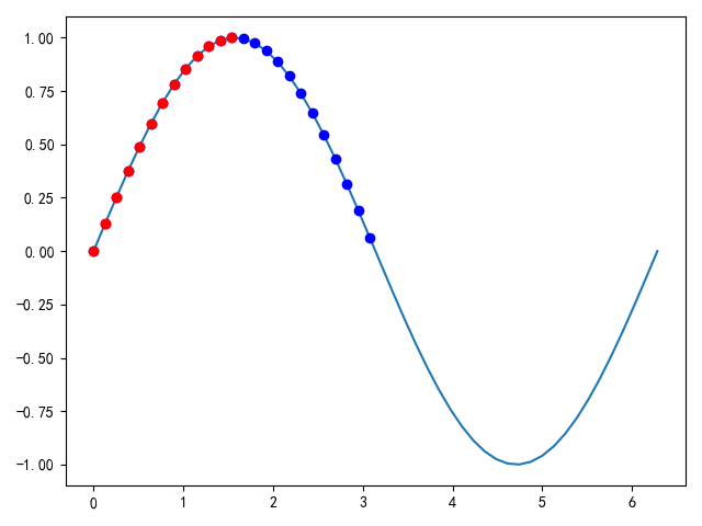
import matplotlib.pyplot as plt

a = np.linspace(0, 2 * np.pi, 50)
b = np.sin(a)
plt.plot(a,b)
mask = b >= 0
plt.plot(a[mask], b[mask], 'bo')
mask = (b >= 0) & (a <= np.pi / 2)
plt.plot(a[mask], b[mask], 'ro')   #后生成的红色点遮挡了原来的蓝色点
plt.show()
缺省索引:
a = np.arange(0, 100, 10)
b = a[:5]
c = a[a >= 50]
print(b) # >>>[ 0 10 20 30 40]
print(c) # >>>[50 60 70 80 90]
where函数: 部分摘自 https://www.cnblogs.com/massquantity/p/8908859.html
用法1:np.where(condition, x, y) #满足condition输出x,不满足输出y 输出数组的结构与条件数组的结构相同
输出结果:array([[1, 8], [3, 4]])
np.where([[True,False],
          [True,True]],    # 官网上的例子
           [[1,2],[3,4]],
           [[9,8], [7,6]])
用法2:np.where(condition)
输出的结果:是满足条件的索引值,输出结果为元组,元组元素的个数=原数组的维数,元组[0]存储的是满足条件的第一维索引值,元组[1]存储的是满足条件的第二维索引值
a=np.arange(0,100,5)
a_1 = a.reshape(4,5)
print(a_1)
'''[[ 0 5 10 15 20]
[25 30 35 40 45]
[50 55 60 65 70]
[75 80 85 90 95]]'''
print(np.where(a_1>10))
'''(array([0, 0, 1, 1, 1, 1, 1, 2, 2, 2, 2, 2, 3, 3, 3, 3, 3], dtype=int32),
array([3, 4, 0, 1, 2, 3, 4, 0, 1, 2, 3, 4, 0, 1, 2, 3, 4], dtype=int32))
'''
切片:
注:从原数组切片后得到的子数组,对子数组的数值修改也会修改原始数组的数值。
import numpy as np

# Create the following rank 2 array with shape (3, 4)
# [[ 1  2  3  4]
#  [ 5  6  7  8]
#  [ 9 10 11 12]]
a = np.array([[1,2,3,4],
              [5,6,7,8],
              [9,10,11,12]])
# [[2 3]
#  [6 7]]
b = a[:2, 1:3]

# A slice of an array is a view into the same data, so modifying it
# will modify the original array.
print(a[0, 1])   # Prints "2"
b[0, 0] = 77     # b[0, 0] is the same piece of data as a[0, 1]
print(a[0, 1])   # Prints "77"      说明是修改的原数组
#----------------------------------------------------------------------------
a = np.array([[1,2,3,4], [5,6,7,8], [9,10,11,12]]row_r1 = a[1, :] # Rank 1 view of the second row of a row_r2 = a[1:2, :] # Rank 2 view of the second row of a print(row_r1, row_r1.shape) # Prints "[5 6 7 8] (4,)" 一维数组 print(row_r2, row_r2.shape) # Prints "[[5 6 7 8]] (1, 4)" 二维数组
#----------------------------------------------------------------------------
#索引取值
import numpy as np

a = np.array([[1,2], [3, 4], [5, 6]])

# An example of integer array indexing.
# The returned array will have shape (3,) and
print(a[[0, 1, 2], [0, 1, 0]])  # Prints "[1 4 5]"

# The above example of integer array indexing is equivalent to this:
print(np.array([a[0, 0], a[1, 1], a[2, 0]]))  # Prints "[1 4 5]"

# When using integer array indexing, you can reuse the same
# element from the source array:
print(a[[0, 0], [1, 1]])  # Prints "[2 2]"

# Equivalent to the previous integer array indexing example
print(np.array([a[0, 1], a[0, 1]]))  # Prints "[2 2]"
#----------------------------------------------------------------------------
# 布尔数值索引
import numpy as np

a = np.array([[1,2], [3, 4], [5, 6]])

bool_idx = (a > 2)   # Find the elements of a that are bigger than 2;
                     # this returns a numpy array of Booleans of the same
                     # shape as a, where each slot of bool_idx tells
                     # whether that element of a is > 2.

print(bool_idx)      # Prints "[[False False]
                     #          [ True  True]
                     #          [ True  True]]"

# We use boolean array indexing to construct a rank 1 array
# consisting of the elements of a corresponding to the True values
# of bool_idx
print(a[bool_idx])  # Prints "[3 4 5 6]"  一维数组

# We can do all of the above in a single concise statement:
print(a[a > 2])     # Prints "[3 4 5 6]"
数组的转置:
import numpy as np

x = np.array([[1,2], [3,4]])
print(x)    # Prints "[[1 2]
            #          [3 4]]"
print(x.T)  # Prints "[[1 3]
            #          [2 4]]"

# Note that taking the transpose of a rank 1 array does nothing:
v = np.array([1,2,3])
print(v)    # Prints "[1 2 3]"
print(v.T)  # Prints "[1 2 3]"
广播:
#不改变原数组
import numpy as np

# We will add the vector v to each row of the matrix x,
# storing the result in the matrix y
x = np.array([[1,2,3],
              [4,5,6],
              [7,8,9],
              [10, 11, 12]])
v = np.array([1, 0, 1])
y = x + v  # Add v to each row of x using broadcasting
print(y)  # Prints "[[ 2  2  4]
          #          [ 5  5  7]
          #          [ 8  8 10]
          #          [11 11 13]]"

 浙公网安备 33010602011771号