【d2l】3.2.线性回归从零实现

【d2l】3.2.线性回归从零实现

生成数据集

本次使用\(\text w [2, -3.4]^\top\)、\(b = 4.2\)和噪声\(\epsilon\)生成数据集和标签

代码中为了简化问题，将标准差设置为0.01

def synthetic_data(w, b, num_examples):
    """生成 y = Xw + b + 噪声"""
    X = torch.normal(0, 1, (num_examples, len(w)))
    y = torch.matmul(X, w) + b

    y += torch.normal(0, 0.01, y.shape)

    return X, y.reshape((-1, 1))

true_w = torch.tensor([2, -3.4])
true_b = 4.2
features, labels = d2l.synthetic_data(true_w, true_b, 1000)

其中features每一行都包含一个二维样本，labels每一行都包含一个标签值（标量）

print(f'features: {features[0]}\nlabel: {labels[0]}')

features: tensor([ 2.1537, -2.2505])
label: tensor([16.1533])

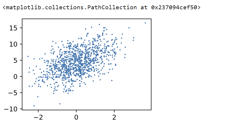
通过生成某一维features和labels的散点图可以直观看出线性关系

d2l.set_figsize()
d2l.plt.scatter(features[:, (0)].detach().numpy(), labels.detach().numpy(), 1)

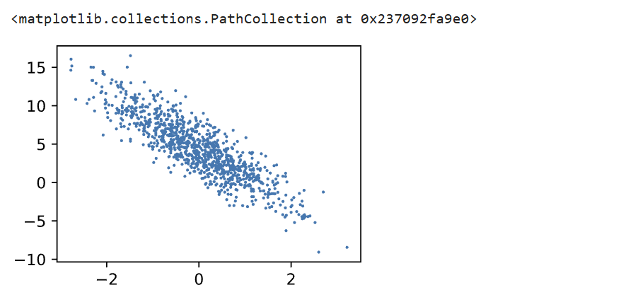
d2l.set_figsize()
d2l.plt.scatter(features[:, (1)].detach().numpy(), labels.detach().numpy(), 1)

读取数据集

由于需要抽取小批量样本来对于模型进行更新，因此有必要定义一个函数来抽取样本

定义一个data_iter函数，该函数接受批量大小、特征矩阵和标签向量作为输入，生成大小为batch_size的小批量。每个小批量包含一组特征和标签

def data_iter(batch_size, features, labels):
    num_examples = len(features)
    indices = list(range(num_examples))

    random.shuffle(indices)

    for i in range(0, num_examples, batch_size):
        batch_indices = torch.tensor(indices[i : min(i + batch_size, num_examples)])
        yield features[batch_indices], labels[batch_indices]

以下是一个小型的测试：

batch_size = 10

for X, y in data_iter(batch_size, features, labels):
    print(X, '\n', y)
    break

tensor([[ 0.8772, -1.2216],
        [-1.1384, -0.4372],
        [ 1.3860, -1.8847],
        [ 2.3808, -0.8306],
        [-0.8442, -0.5185],
        [-1.9760,  0.1422],
        [ 2.1241, -0.8893],
        [-1.1176, -0.1472],
        [ 0.8191,  1.1800],
        [-0.6468,  0.6817]]) 
 tensor([[10.1006],
        [ 3.4129],
        [13.3894],
        [11.8007],
        [ 4.2835],
        [-0.2343],
        [11.4744],
        [ 2.4490],
        [ 1.8172],
        [ 0.5862]])

初始化模型参数

在训练之前需要先初始化模型参数

本次实验中从均值为0，标准差为0.01的正态分布中抽取随机数初始化权重，并将偏置初始化为0

并且为了使用自动微分，要设置requires_grad = True

w = torch.normal(0, 0.01, size = (2, 1), requires_grad = True)
b = torch.zeros(1, requires_grad = True)

定义必要组件

首先是定义模型，对于线性回归模型来说就是矩阵-向量乘法后加上偏置

def linreg(X, w, b):
    """线性回归模型"""
    return torch.matmul(X, w) + b

接着是定义损失函数，利用的是均方损失

def squared_loss(y_hat, y):
    """均方损失"""
    return (y_hat - y.reshape(y_hat.shape))**2 / 2

最后定义优化算法，像前文说的是sgd

def sgd(params, lr, batch_size):
    """小批量随机梯度下降"""
    with torch.no_grad():
        for param in params:
            param -= lr * param.grad / batch_size
            param.grad.zero_()

torch.no_grad()指的是在参数更新过程中并不会建立计算图，因为param本身requires_grad = True，如果没有关掉的话会使得乘上lr的行为被记录，这是我们不需要的

然后就是如同之前说的更新方式，注意/batch_size，因为loss本身是在求和后自动微分，因此要消除批量大小对于结果的影响

最后需要梯度清零，因为梯度默认累加，如果不清零会造成事实性错误

训练

训练流程的迭代过程如下：

• 计算梯度
• 更新参数

函数就很好写了

lr = 0.03
num_epochs = 3
net = d2l.linreg
loss = d2l.squared_loss

for epoch in range(num_epochs):
    for X, y in data_iter(batch_size, features, labels):
        l = loss(net(X, w, b), y)

        l.sum().backward()
        d2l.sgd([w, b], lr, batch_size)

        with torch.no_grad():
            train_l = loss(net(features, w, b), labels)
    print(f'epoch {epoch + 1}, loss {float(train_l.mean()) : f}')

结果如下

epoch 1, loss  0.059939
epoch 2, loss  0.000297
epoch 3, loss  0.000055

再观察相对误差

print(f'w的估计误差：{true_w - w.reshape(true_w.shape)}')
print(f'b的估计误差：{true_b - b}')

w的估计误差：tensor([ 0.0013, -0.0007], grad_fn=<SubBackward0>)
b的估计误差：tensor([0.0009], grad_fn=<RsubBackward1>)

简洁实现

事实上一些常用的损失函数、优化算法等都在torch有实现，因此在实际训练过程中调包就行了

（此处为3.3的内容，因此3.3不再单开专题）