

梯度下降算法
梯度下降法在机器学习中常常用来优化损失函数,是一个非常重要的工具,要想弄清楚梯度下降算法首先要引入一些高数的概念
基本概念
方向导数:是一个数;反映的是f(x,y)在P0点沿方向v的变化率。
偏导数:是多个数(每元有一个);是指多元函数沿坐标轴方向的方向导数,因此二元函数就有两个偏导数。
偏导函数:是一个函数;是一个关于点的偏导数的函数。
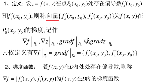
梯度:是一个向量;每个元素为函数对一元变量的偏导数;它既有大小(其大小为最大方向导数),也有方向。
方向导数
方向导数是指函数在某一点沿所给方向的变化率
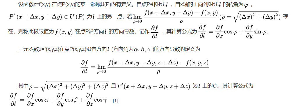
本质就是沿着某一方向函数值的差值/其对应的自变量之间的距离,这个方向是任意的,距离大小相同方向不同由于不同方向的函数变化不同,所以方向导数也不同
梯度
函数z=f(x,y)在点P0处的梯度方向是函数变化率(即方向导数)最大的方向。
梯度的方向就是函数f(x,y)在这点增长最快的方向,梯度的模为方向导数的最大值。
梯度下降法
梯度下降法是一种旨在最小化目标函数(通常是损失函数)的迭代优化算法。其核心思想非常直观:通过计算函数在当前点的梯度(即最陡上升方向),然后沿着梯度的反方向(即最陡下降方向)更新参数,从而逐步逼近函数的局部最小值。这个过程类似于下山时,通过感知最陡的下坡方向一步步走向谷底。作为训练神经网络和许多机器学习模型的基础引擎,它通过不断调整模型参数,使得模型的预测误差越来越小,梯度下降法得到的不一定是全局最优解,类似高中数学中的找极小值点但不一定是最小值点
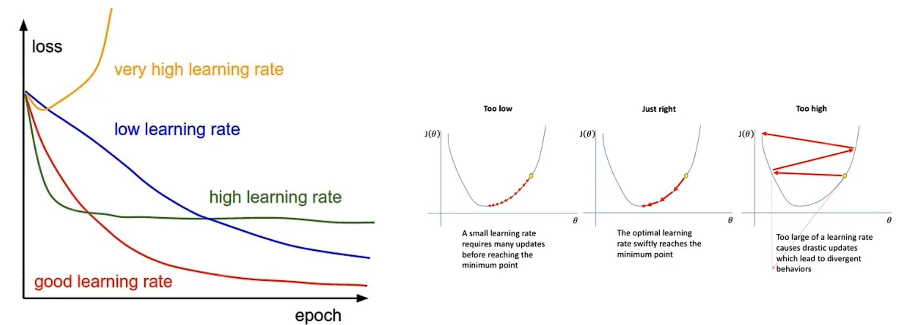
梯度下降算法中有一个重要的叫搜索步长即学习率,该值的人为设定的用于控制每一步的步长,学习率不能太大也不能太小,太大会来回循环难收敛,而太小下降会很慢,效率低
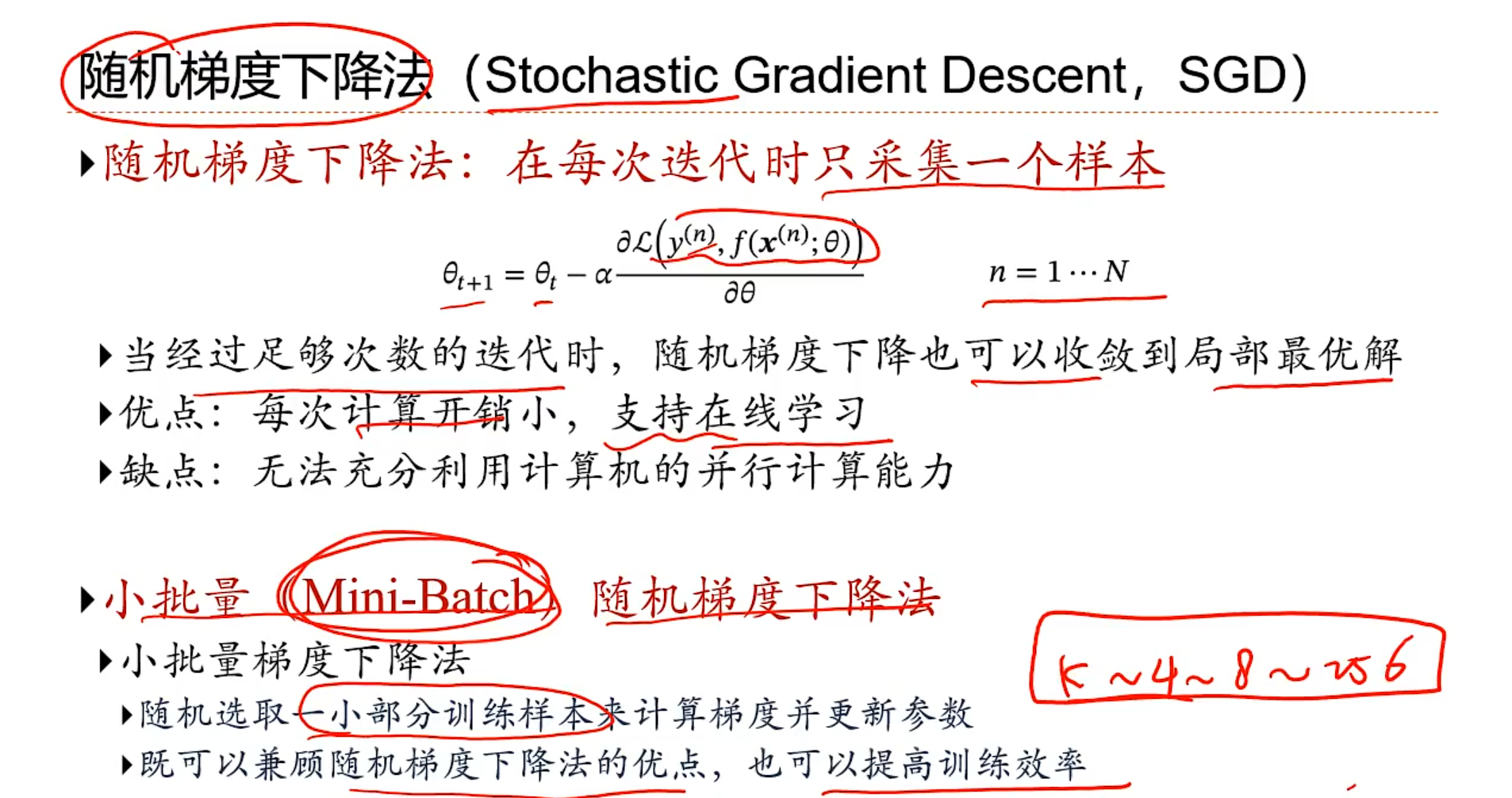
一般在机器学习中,我们会有很多的样本,按照正常的步骤是取所有的样本的平均值来进行梯度下降算法下一个点的选取,但是这样对于计算机性能的要求就很高了们对于CPU消耗很大,算法效率就很低
两种改进策略
python代码实现三种下降算法
import numpy as np
import matplotlib.pyplot as plt
from typing import Tuple, List, Callable, Optional
from dataclasses import dataclass
from enum import Enum


# 定义梯度下降变体类型
# BGD 批量梯度下降算法: 批量梯度下降法是最原始的形式,它是指在每一次迭代时使用所有样本来进行梯度的更新
# SGD 随机梯度下降算法: 随机梯度下降法不同于批量梯度下降,随机梯度下降是在每次迭代时使用一个样本来对参数进行更新(mini-batch size =1)。
# MGD 小批量梯度下降算法: 大多数用于深度学习的梯度下降算法介于以上两者之间,使用一个以上而又不是全部的训练样本。
class GradientDescentVariant(Enum):
    BATCH = "batch"
    STOCHASTIC = "stochastic"
    MINI_BATCH = "mini_batch"

# 记录每次优化之后的结果,变量分别为最优参数向量,损失函数的历史记录,参数向量的历史记录,是否正常收敛,迭代次数
@dataclass
class GradientDescentResult:
    theta: np.ndarray
    loss_history: List[float]
    theta_history: List[np.ndarray]
    converged: bool
    iterations: int


# 优化算法的实现
def gradient_descent(
        x: np.ndarray,
        y: np.ndarray,
        learning_rate: float = 0.01,
        max_iter: int = 1000,
        tol: float = 1e-6,
        batch_size: Optional[int] = None,
        variant: GradientDescentVariant = GradientDescentVariant.BATCH,
        random_state: Optional[int] = None
) -> GradientDescentResult:
    """
    实现梯度下降算法

    参数:
    x: 特征矩阵 (m samples, n features)
    y: 目标向量 (m samples, 1)
    learning_rate: 学习率
    max_iter: 最大迭代次数
    tol: 收敛容差
    batch_size: 小批量大小 (仅用于MINI_BATCH变体)
    variant: 梯度下降变体 (BATCH, STOCHASTIC, MINI_BATCH)
    random_state: 随机种子

    返回:
    GradientDescentResult: 包含结果的对象
    """
    if random_state is not None:
        np.random.seed(random_state)

    m, n = x.shape
    # 添加偏置项, 一个线性方程为f(x) = w0+w1x1+...+wnxn,这里w0由于x0为1,所以需要添加一个常数项
    x_b = np.c_[np.ones((m, 1)), x]

    # 初始化参数
    theta = np.random.randn(n + 1, 1)

    # 存储历史
    loss_history = []
    theta_history = [theta.copy()]

    # 根据变体选择迭代方式
    match variant:
        case GradientDescentVariant.BATCH:
            # 批量梯度下降
            for i in range(max_iter):
                gradients = 2 / m * x_b.T.dot(x_b.dot(theta) - y)
                theta = theta - learning_rate * gradients
                theta_history.append(theta.copy())

                # 计算损失
                loss = np.mean((x_b.dot(theta) - y) ** 2)
                loss_history.append(loss)

                # 检查收敛
                if i > 0 and abs(loss_history[-2] - loss) < tol:
                    return GradientDescentResult(
                        theta=theta,
                        loss_history=loss_history,
                        theta_history=theta_history,
                        converged=True,
                        iterations=i + 1
                    )

        case GradientDescentVariant.STOCHASTIC:
            # 随机梯度下降
            for i in range(max_iter):
                # 随机选择一个样本
                random_index = np.random.randint(m)
                xi = x_b[random_index:random_index + 1]
                yi = y[random_index:random_index + 1]

                gradients = 2 * xi.T.dot(xi.dot(theta) - yi)
                theta = theta - learning_rate * gradients
                theta_history.append(theta.copy())

                # 计算全部数据的损失(用于监控)
                loss = np.mean((x_b.dot(theta) - y) ** 2)
                loss_history.append(loss)

                # 检查收敛
                if i > 0 and abs(loss_history[-2] - loss) < tol:
                    return GradientDescentResult(
                        theta=theta,
                        loss_history=loss_history,
                        theta_history=theta_history,
                        converged=True,
                        iterations=i + 1
                    )

        case GradientDescentVariant.MINI_BATCH:
            # 小批量梯度下降
            if batch_size is None:
                batch_size = min(32, m)  # 默认批量大小

            for i in range(max_iter):
                # 随机选择一个小批量
                indices = np.random.choice(m, batch_size, replace=False)
                x_b_batch = x_b[indices]
                y_batch = y[indices]

                gradients = 2 / batch_size * x_b_batch.T.dot(x_b_batch.dot(theta) - y_batch)
                theta = theta - learning_rate * gradients
                theta_history.append(theta.copy())

                # 计算全部数据的损失(用于监控)
                loss = np.mean((x_b.dot(theta) - y) ** 2)
                loss_history.append(loss)

                # 检查收敛
                if i > 0 and abs(loss_history[-2] - loss) < tol:
                    return GradientDescentResult(
                        theta=theta,
                        loss_history=loss_history,
                        theta_history=theta_history,
                        converged=True,
                        iterations=i + 1
                    )

    # 如果达到最大迭代次数但未收敛
    return GradientDescentResult(
        theta=theta,
        loss_history=loss_history,
        theta_history=theta_history,
        converged=False,
        iterations=max_iter
    )


def create_sample_data(n_samples: int = 100, noise: float = 1.0, random_state: int = 42) -> Tuple[
    np.ndarray, np.ndarray]:
    """创建示例数据"""
    np.random.seed(random_state)
    x = 2 * np.random.rand(n_samples, 1)
    y = 4 + 3 * x + noise * np.random.randn(n_samples, 1)
    return x, y


def plot_results(x: np.ndarray, y: np.ndarray, result: GradientDescentResult, variant: GradientDescentVariant):
    """绘制结果"""
    x_b = np.c_[np.ones((len(x), 1)), x]

    fig, axes = plt.subplots(1, 2, figsize=(12, 4))

    # 子图1: 数据点和拟合线
    axes[0].scatter(x, y, alpha=0.7)
    x_plot = np.linspace(0, 2, 100)
    x_plot_b = np.c_[np.ones((100, 1)), x_plot.reshape(-1, 1)]
    y_plot = x_plot_b.dot(result.theta)
    axes[0].plot(x_plot, y_plot, 'r-', linewidth=2)
    axes[0].set_xlabel('x')
    axes[0].set_ylabel('y')
    axes[0].set_title(f'{variant.value.capitalize()} Gradient Descent Fit')

    # 子图2: 损失函数下降曲线
    axes[1].plot(range(len(result.loss_history)), result.loss_history)
    axes[1].set_xlabel('Iterations')
    axes[1].set_ylabel('Loss')
    axes[1].set_title('Loss Function')
    axes[1].set_yscale('log')

    plt.tight_layout()
    plt.show()


def plot_optimization_path(x: np.ndarray, y: np.ndarray, result: GradientDescentResult):
    """绘制优化路径"""
    x_b = np.c_[np.ones((len(x), 1)), x]
    m = len(y)

    # 创建参数空间网格
    theta0_vals = np.linspace(2, 6, 100)
    theta1_vals = np.linspace(2, 4, 100)
    theta0_mesh, theta1_mesh = np.meshgrid(theta0_vals, theta1_vals)

    # 计算损失曲面
    loss_vals = np.zeros_like(theta0_mesh)
    for i in range(theta0_vals.shape[0]):
        for j in range(theta1_vals.shape[0]):
            theta_val = np.array([[theta0_vals[i]], [theta1_vals[j]]])
            loss_vals[i, j] = (1 / m) * np.sum((x_b.dot(theta_val) - y) ** 2)

    # 提取参数历史
    theta0_history = [theta[0, 0] for theta in result.theta_history]
    theta1_history = [theta[1, 0] for theta in result.theta_history]

    # 绘制等高线图和优化路径
    plt.figure(figsize=(10, 8))
    contour = plt.contour(theta0_mesh, theta1_mesh, loss_vals, levels=50, cmap='viridis')
    plt.clabel(contour, inline=True, fontsize=8)
    plt.plot(theta0_history, theta1_history, 'r.-', markersize=5, linewidth=1)
    plt.plot(theta0_history[-1], theta1_history[-1], 'ro', markersize=8, label='Final')
    plt.plot(theta0_history[0], theta1_history[0], 'go', markersize=8, label='Start')
    plt.xlabel('θ₀')
    plt.ylabel('θ₁')
    plt.title('Gradient Descent Optimization Path')
    plt.colorbar(contour)
    plt.legend()
    plt.show()


def compare_variants(x: np.ndarray, y: np.ndarray):
    """比较不同梯度下降变体"""
    variants = [
        (GradientDescentVariant.BATCH, "Batch GD"),
        (GradientDescentVariant.STOCHASTIC, "Stochastic GD"),
        (GradientDescentVariant.MINI_BATCH, "Mini-Batch GD")
    ]

    plt.figure(figsize=(10, 6))

    for variant, label in variants:
        if variant == GradientDescentVariant.MINI_BATCH:
            result = gradient_descent(x, y, learning_rate=0.1, variant=variant, batch_size=20, random_state=42)
        else:
            result = gradient_descent(x, y, learning_rate=0.1, variant=variant, random_state=42)

        plt.plot(range(len(result.loss_history)), result.loss_history, label=label)

    plt.xlabel('Iterations')
    plt.ylabel('Loss')
    plt.title('Comparison of Gradient Descent Variants')
    plt.yscale('log')
    plt.legend()
    plt.grid(True)
    plt.show()


# 主程序
if __name__ == "__main__":
    # 创建示例数据
    x, y = create_sample_data(n_samples=100, noise=1.0)

    # 测试批量梯度下降
    print("Running Batch Gradient Descent...")
    batch_result = gradient_descent(x, y, learning_rate=0.1, variant=GradientDescentVariant.BATCH, random_state=42)
    print(f"Converged: {batch_result.converged}, Iterations: {batch_result.iterations}")
    print(f"Final parameters: θ₀ = {batch_result.theta[0, 0]:.4f}, θ₁ = {batch_result.theta[1, 0]:.4f}")
    plot_results(x, y, batch_result, GradientDescentVariant.BATCH)
    plot_optimization_path(x, y, batch_result)

    # 测试随机梯度下降
    print("\nRunning Stochastic Gradient Descent...")
    stochastic_result = gradient_descent(x, y, learning_rate=0.1, variant=GradientDescentVariant.STOCHASTIC,
                                         random_state=42)
    print(f"Converged: {stochastic_result.converged}, Iterations: {stochastic_result.iterations}")
    print(f"Final parameters: θ₀ = {stochastic_result.theta[0, 0]:.4f}, θ₁ = {stochastic_result.theta[1, 0]:.4f}")
    plot_results(x, y, stochastic_result, GradientDescentVariant.STOCHASTIC)

    # 测试小批量梯度下降
    print("\nRunning Mini-Batch Gradient Descent...")
    mini_batch_result = gradient_descent(x, y, learning_rate=0.1, variant=GradientDescentVariant.MINI_BATCH,
                                         batch_size=20, random_state=42)
    print(f"Converged: {mini_batch_result.converged}, Iterations: {mini_batch_result.iterations}")
    print(f"Final parameters: θ₀ = {mini_batch_result.theta[0, 0]:.4f}, θ₁ = {mini_batch_result.theta[1, 0]:.4f}")
    plot_results(x, y, mini_batch_result, GradientDescentVariant.MINI_BATCH)

    # 比较不同变体
    compare_variants(x, y)
 浙公网安备 33010602011771号