系统树图 | Dendrogram construction | Phylogenetic Analysis | Cladogram | 进化分枝图 | TreeExp
使用基因表达的数据来做tree
TreeExp这个包的核心代码很少很少,借用里面的几个函数即可。
使用scale后的data,列是sample,行是gene
# add mix as a reference
merged.exprM.scale$Mixed <- rowSums(merged.exprM.scale)

# important, rm NA
merged.exprM.scale[is.na(merged.exprM.scale)] <- 0

library(TreeExp)
disM <- dist.euc(merged.exprM.scale)
dim(disM)

rownames(disM) <- colnames(merged.exprM.scale)
colnames(disM) <- colnames(merged.exprM.scale)

disM[is.na(disM)] <- 0

tr <- NJ(disM)
tr$tip.label

tr <- ape::root(tr, outgroup = "Mixed")

options(repr.plot.width=6, repr.plot.height=4)
plot(tr, show.node.label = TRUE)
绘图
library("ggtree")
library(RColorBrewer)
tmp.colors <- c(brewer.pal(9,"Set1")[c(1:5,7:9)],"black")

options(repr.plot.width=6, repr.plot.height=3)
ggtree(tr, branch.length="none", linetype = "solid", size = 1) +
  # theme_tree2() +
  # vjust: + -> down; hjust: + -> left
  geom_tiplab(size=4, color=tmp.colors, align=F, hjust = 0.8, vjust = 2, angle = 30, fontface = "bold") +
  #scale_y_continuous(limits = c(0, 5)) +
  coord_flip() +
  scale_x_reverse(expand = c(0,3)) +
  labs(x = "", y = "", title = "ENCC Cladogram") +
  theme(plot.title = element_text(hjust = 0.5, vjust = -5, face = "bold", size=20))

ggsave(filename = "manuscript/HSCR.Cladogram.pdf", width = 6, height = 3)
参考path:EllyLab/human/singleCell/HSCR/HSCR_additional_analysis.ipynb
Molecular Architecture of the Mouse Nervous System
表示亲缘关系的树状图解
先看文章里是怎么做的:
Dendrogram construction
All linkage and distance calculations were performed after Log2 transformation. log2转换,很好理解。
The starting point of the dendrogram construction was the 265 clusters. 这里使用了所有的cluster。
For each gene, we computed average expression, trinarization with f = 0.2, trinarization with f = 0.05 and enrichment score. 这里应该是对每一个gene,计算在每一个cluster里的平均表达,trinarization和富集得分。
For each cluster we also know the number of cells, annotations, tissue distribution and samples of origin. We defined major classes of cell types based on prior knowledge: neurons, astroependymal, oligodendrocytes, vascular (without VLMC), immune cells and neural crest-like. 每个类已经有比较好的注释了。
For each class, we defined pan-enriched genes based on the trinarization 5% score. Each class (except neurons) was tested against neurons, to find all the genes where the fraction of clusters with trinarization score = 1 in the class was greater than the fraction of clusters with trinarization score > 0.9 among neurons. 定义了pan-enriched genes
In order to suppress batch effects (mainly due to ambient oligodenderocyte RNA in hindbrain and spinal cord samples), we collected the unique set of genes pan-enriched in the non-neuronal clusters, as well as a set of non-neuronal genes that we believe to have tendency to appear in floating RNA (Trf, Plp1, Mog, Mobp, Mfge8, Mbp, Hbb-bs, H2-DMb2) and a set of immediate early genes (Fos, Jun, Junb, Egr1). These genes were set to zero within the neuronal clusters to avoid any batch effect when clustering the neuronal clusters. 去掉批次效应
We further removed sex specific genes (Xist, Tsix, Eif2s3y, Ddx3y, Uty, and Kdm5d) and immediate early genes Egr1 and Jun from all clusters. We bounded the number of detected genes in each cluster to the top 5000 genes expressed, followed by scaling the total sum of each cluster profile to 10,000. 去掉性别基因
Next, we selected genes for linkage analysis: from each cluster select the top N = 28 enriched genes (based on pre-calculated enrichment score), perform initial clustering using linkage (Euclidean distance, Ward in MATLAB), and cut the tree based on distance criterion 50. This clustering aimed to capture the coarse structure of the hierarchy. 初步筛选基因
For each of the resulting clusters, we calculated the enrichment score as the mean over the cluster divided by the total sum and selected the 1.5 N top genes. These were added to the previously selected genes. 添加基因
Finally, we built the dendrogram using linkage (correlation distance and Ward method). 最终用MATLAB的linkage包来作图。
如何选择基因和整合基因才是绘制dendrogram的核心。
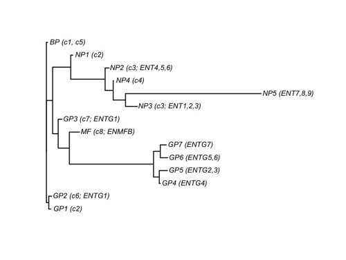
这不是最优的作图,每个支的长短应该不一样,以表示发育的距离。
TreeExp计算,R默认plot函数成图效果非常好:
参考:
Phylogenetic Analysis of Gene Expression
Estimating the strength of expression conservation from high throughput RNA-seq data sci-hub
TreeExp - github
Data Integration, Manipulation and Visualization of Phylogenetic Trees - Guangchuang Yu


 浙公网安备 33010602011771号