Deep Learning1:Sparse Autoencoder
学习stanford的课程http://ufldl.stanford.edu/wiki/index.php/UFLDL_Tutorial 一个月以来,对算法一知半解,Exercise也基本上是复制别人代码,现在想总结一下相关内容
1. Autoencoders and Sparsity
稀释编码:Sparsity parameter
隐藏层的平均激活参数为
![\begin{align}
\hat\rho_j = \frac{1}{m} \sum_{i=1}^m \left[ a^{(2)}_j(x^{(i)}) \right]
\end{align}](http://ufldl.stanford.edu/wiki/images/math/8/7/2/8728009d101b17918c7ef40a6b1d34bb.png)
约束为

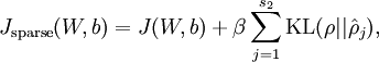
为实现这个目标,在cost Function上额外加上一项惩罚系数
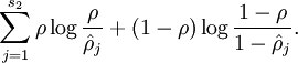
当此项达到最小值
此时cost Function
同时为了方便编程,将隐藏层时的后向传播参数也增加一项
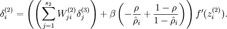
为了得到Sparsity parameter,先对所有训练数据进行前向步骤,从而得到激活参数,再次前向步骤,进行反向传播调参,也就是要对所有训练数据进行两次的前向步骤
2.Backpropagation Algorithm
在计算过程中,简化了计算步骤
对于训练集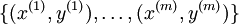 ,cost Function如下
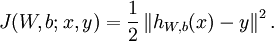
仅含方差项
![\begin{align}
J(W,b)
&= \left[ \frac{1}{m} \sum_{i=1}^m J(W,b;x^{(i)},y^{(i)}) \right]
+ \frac{\lambda}{2} \sum_{l=1}^{n_l-1} \; \sum_{i=1}^{s_l} \; \sum_{j=1}^{s_{l+1}} \left( W^{(l)}_{ji} \right)^2
\\
&= \left[ \frac{1}{m} \sum_{i=1}^m \left( \frac{1}{2} \left\| h_{W,b}(x^{(i)}) - y^{(i)} \right\|^2 \right) \right]
+ \frac{\lambda}{2} \sum_{l=1}^{n_l-1} \; \sum_{i=1}^{s_l} \; \sum_{j=1}^{s_{l+1}} \left( W^{(l)}_{ji} \right)^2
\end{align}](http://ufldl.stanford.edu/wiki/images/math/4/5/3/4539f5f00edca977011089b902670513.png)
第一部分是方差,第二部分是规范化项,也称为weight decay项,此公式为overall cost function
参数W,b的迭代公式如下
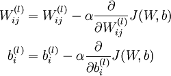
α为学习率
那么,backpropagation algorithm在参数计算中极大提高了效率
目的:梯度下降法,迭代多次,得到优化参数
每次迭代都计算cost function和gradient,再进行下一次迭代
BP 前向传播后,定义误差项1.输出层是对cost function 对输出结果求导2.中间层 下一层误差项与网络系数相乘,实现逆向推导
cost function分别对W,b求导如下
![\begin{align}
\frac{\partial}{\partial W_{ij}^{(l)}} J(W,b) &=
\left[ \frac{1}{m} \sum_{i=1}^m \frac{\partial}{\partial W_{ij}^{(l)}} J(W,b; x^{(i)}, y^{(i)}) \right] + \lambda W_{ij}^{(l)} \\
\frac{\partial}{\partial b_{i}^{(l)}} J(W,b) &=
\frac{1}{m}\sum_{i=1}^m \frac{\partial}{\partial b_{i}^{(l)}} J(W,b; x^{(i)}, y^{(i)})
\end{align}](http://ufldl.stanford.edu/wiki/images/math/9/3/3/93367cceb154c392aa7f3e0f5684a495.png)
首先,对训练对象进行前向网络激活运算,得到网络输入值hW,b(x)
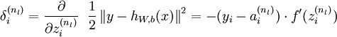
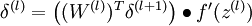
接着,对网络层l 中每一个节点i ,计算误差项 ,衡量该节点对于输出的误差所占权重,可用网络激活输出值与真实目标值之差来定义
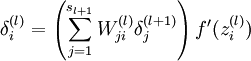
 ,nl 是输出层,对于隐藏层,则用
 作为输出的误差项的权重比来定义
算法步骤如下
- Perform a feedforward pass, computing the activations for layers L2, L3, and so on up to the output layer
![L_{n_l}]() .
. - For each output unit i in layer nl (the output layer), set
- For
![l = n_l-1, n_l-2, n_l-3, \ldots, 2]()
- For each node i in layer l, set
- For each node i in layer l, set
- Compute the desired partial derivatives, which are given as:
 .
.

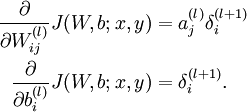
对于矩阵,在MATLAB中如下
- Perform a feedforward pass, computing the activations for layers
![\textstyle L_2]() ,
, ![\textstyle L_3]() , up to the output layer
, up to the output layer ![\textstyle L_{n_l}]() , using the equations defining the forward propagation steps
, using the equations defining the forward propagation steps - For the output layer (layer
![\textstyle n_l]() ), set
), set - For
![\textstyle l = n_l-1, n_l-2, n_l-3, \ldots, 2]()
- Set
- Set
- Compute the desired partial derivatives:
 ,
, , up to the output layer
 , using the equations defining the forward propagation steps
 ), set

注: 为sigmoid函数,则
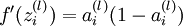
在此基础上,梯度下降算法gradient descent algorithm步骤如下
- Set
![\textstyle \Delta W^{(l)} := 0]() ,
, ![\textstyle \Delta b^{(l)} := 0]() (matrix/vector of zeros) for all
(matrix/vector of zeros) for all ![\textstyle l]() .
. - For
![\textstyle i = 1]() to
to ![\textstyle m]() ,
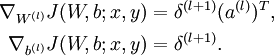
,- Use backpropagation to compute
![\textstyle \nabla_{W^{(l)}} J(W,b;x,y)]() and
and ![\textstyle \nabla_{b^{(l)}} J(W,b;x,y)]() .
. - Set
![\textstyle \Delta W^{(l)} := \Delta W^{(l)} + \nabla_{W^{(l)}} J(W,b;x,y)]() .
. - Set
![\textstyle \Delta b^{(l)} := \Delta b^{(l)} + \nabla_{b^{(l)}} J(W,b;x,y)]() .
.
- Use backpropagation to compute
- Update the parameters:
 ,
,
 .
.
 ,
,
 .
. .
. .
.![\begin{align}
W^{(l)} &= W^{(l)} - \alpha \left[ \left(\frac{1}{m} \Delta W^{(l)} \right) + \lambda W^{(l)}\right] \\
b^{(l)} &= b^{(l)} - \alpha \left[\frac{1}{m} \Delta b^{(l)}\right]
\end{align}](http://ufldl.stanford.edu/wiki/images/math/0/f/7/0f7430e97ec4df1bfc56357d1485405f.png)
3.Visualizing a Trained Autoencoder
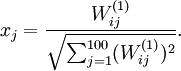
用pixel intensity values可视化编码器
已知输出
约束
定义pixel  (for all 100 pixels,
  )
)
posted on 2016-10-13 16:18 Beginnerpatienceless 阅读(283) 评论(0) 收藏 举报

 浙公网安备 33010602011771号