手写数字识别——手动搭建全连接层

本文使用TensorFlow2.0手动搭建简单的全连接网络进行MNIST手写数据集的分类识别，逐步讲述实现过程，穿插TensorFlow2.0语法，文末给出完整的代码。废话少说，开始动手吧！

 

 

一、量子波动撸代码

该节先给出各代码片段，第二节将这些片段汇总成程序，这些代码片段故意包含了一些错误之处，在第二节中会进行一一修正。如要正确的代码，请直接参考第三节。如若读者有一番闲情逸致，可跟随笔者脚步，看看自己是否可以事先发现这些错误。

首先，导入依赖的两个模块，一个是tensorflow，另一个是tensorflow.keras.datasets，我们要的数据集MNIST就是由这个datasets管理下载的。https://tensorflow.google.cn/datasets/catalog/overview?hl=en中列出了datasets管理的所有数据集。

import tensorflow as tf
#数据集管理器
from tensorflow.keras import datasets

 

导入数据集，数据集一般由训练数据和测试数据构成，用（x,y）存储训练图片和标签，用（val_x,val_y）存储测试图片和标签。

(x,y),(val_x,val_y) = datasets.mnist.load_data()

 

在导入后，需要对数据形式进行初步查看，对于图像识别来说，图片的数量、大小、通道数量和数据范围、类型是必须了解的。以一下程序能打印出这些信息，注释为输出结果。由结果可知，datasets导出的数据是Numpy数组，类型为uint8，训练图片共60k张，大小为28*28，为灰度图像，灰度范围0~255；测试图片共10k张。

print(type(x),x.dtype)  　　　　　　#<class 'numpy.ndarray'> uint8
print(type(y),y.dtype)  　　　　　　#<class 'numpy.ndarray'> uint8
print(x.shape,y.shape)  　　　　　　#(60000, 28, 28) (60000,)
print(val_x.shape,val_y.shape)    #(10000, 28, 28) (10000,)
print(x.max(),x.min())　　　　　　　#255 0
print(y.max(),y.min())　　　　　　　#9 0

 

在训练前必须先将数据转为Tensor。用tf.convert_to_tensor(value,dtype)函数可将value转为Tensor，并可指定数据类型（dtype）。将x,val_x转成浮点类型，而训练数据的标签y需要先转为Tensor整型再转化为独热码形式，测试数据val_y的标签转化为Tensor整型，独热码转换可用tf.one_hot(indices,depth,dtype)，indices必须是整型，这也就是为什么先转成Tensor整型的原因，depth决定独热码位数，dtype默认是tf.float32。以下代码完成数据类型转换。

#需要将数据转成Tensor
x = tf.convert_to_tensor(x,dtype=tf.float32)
y = tf.convert_to_tensor(y,dtype=tf.int32)
val_x = tf.convert_to_tensor(val_x,dtype=tf.float32)    
val_y = tf.convert_to_tensor(val_y,dtype=tf.int32)
#独热码
y = tf.one_hot(y,depth=10)
print(y.shape) #(60000, 10)

 

对于如此庞大的数据集，直接一次性加载到内存进行计算是不现实的，所以采用批处理的方式将数据集分批喂进网络，在分批前先对数据shuffle一下，以防网络发现顺序规律。事实上，把整个数据集一次喂给网络来更新参数的过程称为批梯度下降；而每次只喂一张图片，则称为随机梯度下降；每次将一小批图片喂给网络，称为小批量梯度下降。关于三者的区别可以参考https://www.cnblogs.com/lliuye/p/9451903.html。简单来说，小批量梯度下降是最合适的，一般Batch设的较大，则达到最大准确率的速度变慢，但更容易收敛；Batch设小了，在一开始，准确率提高得非常快，但是最终收敛可能不太好。

test_db =  tf.data.Dataset.from_tensor_slices((val_x,val_y)).shuffle(10000).batch(256)
train_db =  tf.data.Dataset.from_tensor_slices((x,y)).shuffle(10000).batch(256)

 

 train_db是可以直接迭代的，下面进行一次迭代，观察迭代结果，可以知道每一次迭代图片数量就是Batch大小。

train_iter = iter(train_db)
sample = next(train_iter)
print(sample[0].shape,sample[1].shape)  #(256, 28, 28) (256, 10)

 

 

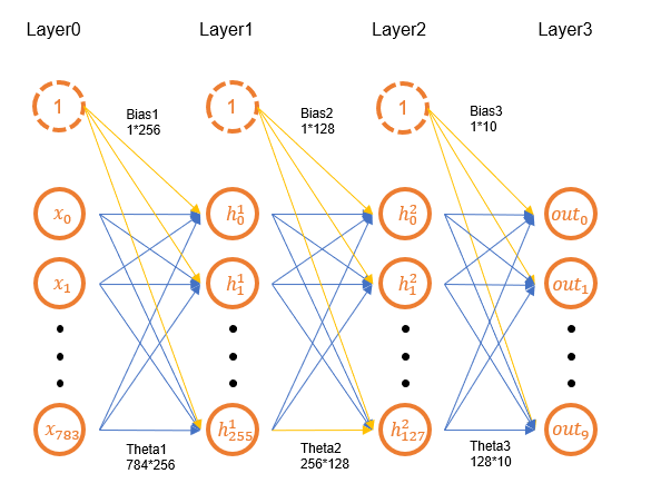
下面就可以开始构建全连接网络了，结构如上图所示。网络节点数为784（input）->256->128->10(output)，加上输入输出一共4层，其中输入层是打平后的图片，共28*28=784个像素；输出层由类别数决定，这里手写数字0~9共10类，故输出有10个节点，这些节点表示属于该类的概率。构建网络需要有初始化的参数，可以利用高斯分布进行参数的初始化，即函数tf.random.normal(shape,mean=0.0,stddev=1.0)，但是为了避免参数初始化过大，常采用截断型正态分布，即函数tf.random.truncated_normal(shape,mean=0.0,stddev=1.0)，该函数将丢弃幅度大于平均值的2个标准偏差的值并重新选择，这里也就是说随机的值范围在-2~2之间。在初始化参数时也要注意参数的shape，例如784->256的参数shape应为(784,256)，偏置shape应为(256,)，这样还方便之后的矩阵运算。偏置一般都初始化为0。此外，所有参数都必须转为tf.Variable类型，才可以记录下梯度信息。

#input(layer0)->layer1: nodes:784->256
theta_1 = tf.Variable(tf.random.truncated_normal([784,256]))#因为后面要记录梯度信息，所以要用Varible
bias_1  = tf.Variable(tf.zeros([256]))

#layer1->layer2: nodes:256->128
theta_2 = tf.Variable(tf.random.truncated_normal([256,128]))
bias_2  = tf.Variable(tf.zeros([128]))

#layer2->out(layer3): nodes:128->10
theta_3 = tf.Variable(tf.random.truncated_normal([128,10]))
bias_3  = tf.Variable(tf.zeros([10]))

初始化参数后，可以统计一下网络的参数量：784*256+256*128+128*10+256+128+10=235146。大约20万个参数，相比一些经典卷积网络，全连接网络的参数量还是比较少的。

 

对train_db进行迭代，套上enumerate()以便获取迭代批次。每一批数据，都要进行前向传播。首先，将shape为[256,28,28]图片打平为[256,784]，这个可以借助tf.reshape(tensor,shape)，在不改变元素个数的前提下，对维度进行分解或者合并。这样，h_1=x@theta1+bias1就可以得到下一层网络的节点值。h_1的shape为[256,256]；同理，h_2的shape为[256,128]，h_3的shape为[256,10]。每一层计算之后都应该加上一个激活函数，最常用的就是ReLu，通过激活函数可以增加网络的非线性表达能力，这里使用函数tf.nn.relu(features)。

由于更新参数需要得到各参数的梯度信息，因此前向传播要用with tf.GradientTape() as tape:包裹起来，关于with as 的语法如果不熟悉可以参考https://www.cnblogs.com/DswCnblog/p/6126588.html。此外，还得计算代价函数，就是Loss，一般采用差平方的均值来计算，差平方使用tf.math.square(x)，均值采用tf.math.reduce_mean(input_tensor,axis=None)，如果不指定axis就对所有元素求均值，返回值是标量，而如果指定axis，就仅对该axis做均值，结果的shape中该axis消失。

for batch, (x, y) in enumerate(train_db):
    # x:[256,28,28]
    x = tf.reshape(x, [-1, 28 * 28])  # 最后一批<256个,用-1可以自动计算
    with tf.GradientTape() as tape:
        # 前向传播
        # x:[256,784] theta_1:[784,256] bias_1:[256,] h_1:[256,256]
        h_1 = x @ theta_1 + bias_1
        h_1 = tf.nn.relu(h_1)
        # h_1:[256,256] theta_2:[256,128] bias_2:[128,] h_2:[256,128]
        h_2 = h_1 @ theta_2 + bias_2
        h_2 = tf.nn.relu(h_2)
        # h_2:[256,128] theta_3:[128,10] bias_2:[10,] out:[256,10]
        out = h_2 @ theta_3 + bias_3# 计算代价函数
        # out:[256,10] y:[256,10]
        loss = tf.math.square(y - out)
        # loss:[256,10]->scalar
        loss = tf.math.reduce_mean(loss)

 

上一部分对梯度信息进行了记录，我们要更新参数，必须先执行loss对各参数求导，之后根据学习率进行参数更新：

alpha = tf.constant(1e-3)
#获取梯度信息，grads为一个列表，顺序依据给定的参数列表
grads = tape.gradient(loss,[theta_1,bias_1,theta_2,bias_2,theta_3,bias_3])
#根据给定列表顺序，对参数求导
theta_1 = theta_1 - alpha * grads[0]
theta_2 = theta_2 - alpha * grads[2]
theta_3 = theta_3 - alpha * grads[4]
bias_1 = bias_1 - alpha * grads[1]
bias_2 = bias_2 - alpha * grads[3]
bias_3 = bias_3 - alpha * grads[5]
#每隔100个batch打印一次loss
if batch % 100 ==0:
    print(batch,'loss:',float(loss))

 

到此为止，整个训练网络就完成了。为了测试网络的效果，我们需要对测试数据集进行预测，并且计算出准确率。关于测试的前向传播同之前的一样，但测试时并不需要对参数进行更新。网络的输出层有10个类别的概率，我们要取概率最大的作为预测的类别，这可以通过tf.math.argmax(input,axis=None)来实现，该函数可以返回数组中最大数的位置，axis的作用类似与reduce_mean。预测结果的正确与否可用tf.math.equal(x,y)来判别，它返回Bool型列表。由于一批次有256个图片，那么预测结果也有256个，可以用tf.math.reduce_sum(input_tensor,axis=None)进行求和，求和前通过tf.cast(x,dtype)将Bool类型转为整型。

correct_cnt = 0  # 预测对的数量
total_val = val_y.shape[0]  # 测试样本总数

# 测试数据预测
for (val_x, val_y) in test_db:
    val_x = tf.reshape(val_x, [-1, 28 * 28])
    val_h_1 = val_x @ theta_1 + bias_1
    val_h_1 = tf.nn.relu(val_h_1)
    val_h_2 = val_h_1 @ theta_2 + bias_2
    val_h_2 = tf.nn.relu(val_h_2)
    val_out = val_h_2 @ theta_3 + bias_3

    # val_out:(256,10) pred:(256,)
    pred = tf.math.argmax(val_out, axis=-1)
    # acc:bool (256,)
    acc = tf.math.equal(pred, val_y)
    acc = tf.cast(acc, dtype=tf.int32)
    correct_cnt += tf.math.reduce_sum(acc)

percent = float(correct_cnt / total_val)
print('val_acc:',percent)

 

自此所有的代码片段都已分析完毕。下一节将展示综合的代码和运行结果。

 

 

 

 

二、亡羊补牢，搞定BUG

为了之后叙述的方便，这里先给出综合的代码，在原有基础上，还加上了训练集的准确度计算，和时间记录。

import tensorflow as tf
#数据集管理器
from tensorflow.keras import datasets
import time

#导入数据集
(x,y),(val_x,val_y) = datasets.mnist.load_data()
#数据集信息
print('type_x:',type(x),'dtype_x:',x.dtype)
print('type_y:',type(y),'dtype_y:',y.dtype)
print('shape_x:',x.shape,'shape_y:',y.shape)
print('shape_val:',val_x.shape,'shape_val:',val_y.shape)
print('max_x:',x.max(),'min_x:',x.min())
print('max_y:',y.max(),'min_y:',y.min())

#需要将数据转成Tensor
x = tf.convert_to_tensor(x,dtype=tf.float32)
y = tf.convert_to_tensor(y,dtype=tf.int32)
val_x = tf.convert_to_tensor(val_x,dtype=tf.float32)
val_y = tf.convert_to_tensor(val_y,dtype=tf.int32)
#独热码
y = tf.one_hot(y,depth=10)
print('one_hot_y:',y.shape)

#生成批处理
test_db =  tf.data.Dataset.from_tensor_slices((val_x,val_y)).shuffle(10000).batch(256)
train_db =  tf.data.Dataset.from_tensor_slices((x,y)).shuffle(10000).batch(256)
#批处理数据信息
train_iter = iter(train_db)
sample = next(train_iter)
print('sample_x_shape:',sample[0].shape,'sample_y_shape:',sample[1].shape)

#参数初始化
#input(layer0)->layer1: nodes:784->256
theta_1 = tf.Variable(tf.random.truncated_normal([784,256]))#因为后面要记录梯度信息，所以要用Varible
bias_1  = tf.Variable(tf.zeros([256]))

#layer1->layer2: nodes:256->128
theta_2 = tf.Variable(tf.random.truncated_normal([256,128]))
bias_2  = tf.Variable(tf.zeros([128]))

#layer2->out(layer3): nodes:128->10
theta_3 = tf.Variable(tf.random.truncated_normal([128,10]))
bias_3  = tf.Variable(tf.zeros([10]))

#确定学习率
alpha = tf.constant(1e-3)
# 测试样本总数
total_val = val_y.shape[0]
# 训练样本总数
total_y = y.shape[0]
#开始时间
start_time = time.time()

for echo in range(500):
    #前向传播
    correct_cnt = 0       # 预测对的数量

    for batch, (x, y) in enumerate(train_db):
        # x:[256,28,28]
        x = tf.reshape(x, [-1, 28 * 28])  # 最后一批<256个,用-1可以自动计算
        with tf.GradientTape() as tape:
            # 前向传播
            # x:[256,784] theta_1:[784,256] bias_1:[256,] h_1:[256,256]
            h_1 = x @ theta_1 + bias_1
            h_1 = tf.nn.relu(h_1)
            # h_1:[256,256] theta_2:[256,128] bias_2:[128,] h_2:[256,128]
            h_2 = h_1 @ theta_2 + bias_2
            h_2 = tf.nn.relu(h_2)
            # h_2:[256,128] theta_3:[128,10] bias_2:[10,] out:[256,10]
            out = h_2 @ theta_3 + bias_3
            # 计算代价函数
            # out:[256,10] y:[256,10]
            loss = tf.math.square(y - out)
            # loss:[256,10]->scalar
            loss = tf.math.reduce_mean(loss)

        # 获取梯度信息，grads为一个列表，顺序依据给定的参数列表
        grads = tape.gradient(loss, [theta_1, bias_1, theta_2, bias_2, theta_3, bias_3])
        # 根据给定列表顺序，对参数求导
        theta_1 = theta_1 - alpha * grads[0]
        theta_2 = theta_2 - alpha * grads[2]
        theta_3 = theta_3 - alpha * grads[4]
        bias_1 = bias_1 - alpha * grads[1]
        bias_2 = bias_2 - alpha * grads[3]
        bias_3 = bias_3 - alpha * grads[5]

        pred = tf.math.argmax(out, axis=-1)
        y_label = tf.math.argmax(y, axis=-1)
        acc = tf.math.equal(pred, y_label)
        acc = tf.cast(acc, dtype=tf.int32)
        correct_cnt += tf.math.reduce_sum(acc)

        # 每隔100个batch打印一次loss
        if batch % 100 == 0:
            print(batch, 'loss:', float(loss))

    #训练的准确度
    percent = float(correct_cnt / total_y)
    print('train_acc:', percent)

    correct_cnt = 0  # 预测对的数量


    # 测试数据预测
    for (val_x, val_y) in test_db:
        val_x = tf.reshape(val_x, [-1, 28 * 28])
        val_h_1 = val_x @ theta_1 + bias_1
        val_h_1 = tf.nn.relu(val_h_1)
        val_h_2 = val_h_1 @ theta_2 + bias_2
        val_h_2 = tf.nn.relu(val_h_2)
        val_out = val_h_2 @ theta_3 + bias_3

        # val_out:(256,10) pred:(256,)
        pred = tf.math.argmax(val_out, axis=-1)
        # acc:bool (256,)
        acc = tf.math.equal(pred, val_y)
        acc = tf.cast(acc, dtype=tf.int32)
        correct_cnt += tf.math.reduce_sum(acc)

    #测试准确度
    percent = float(correct_cnt / total_val)
    print('val_acc:', percent)
    print('time:',int(time.time()-start_time)//60,':',int(time.time()-start_time)%60)

 

以为自此万事大吉，没想到刚跑就报错，报错如下：

0 loss: 75169185792.0
Traceback (most recent call last):
File "D:/programe/tensorflow/tf-project/practice01/forward.py", line 76, in <module>
theta_1 = theta_1 - alpha * grads[0]
ValueError: Attempt to convert a value (None) with an unsupported type (<class 'NoneType'>) to a Tensor.

 

由报错可知，错误大概出在参数更新那里。并且此时第一loss已经被打印出来了，虽然这个Loss有点大得离谱，不过应该不会使得theta_1为None或者grads为None。经过Debug确认为grads为None，并且还发现参数经过一次更新后，其类型从Variable变成了普通的Tensor类型。这就说明问题了，Variable在和Tensor计算时会转换成Tensor。之前曾说过，只有Variable才能记录下梯度信息，因此在第二轮更新时，梯度已经不能正常记录了，才导致grads为None。解决的办法有两种，一种在更新后用tf.Variable进行转换；第二种就是使用原地更新，Variable特有方法.assign_sub进行减法运算，除此之外，还有类似的加法运算等。将上面程序的81~86行改成下面程序段：

theta_1.assign_sub(alpha*grads[0])#原地更新，类型不变
theta_2.assign_sub(alpha * grads[2])
theta_3.assign_sub(alpha * grads[4])
bias_1.assign_sub(alpha*grads[1])
bias_2.assign_sub(alpha * grads[3])
bias_3.assign_sub(alpha * grads[5])

 

再次运行程序，且看报错信息：

0 loss: 87516119040.0
100 loss: nan
200 loss: nan
train_acc: 0.09881666666666666
Traceback (most recent call last):
  File "D:/programe/tensorflow/tf-project/practice01/forward.py", line 110, in <module>
    acc = tf.math.equal(pred, val_y)
tensorflow.python.framework.errors_impl.InvalidArgumentError: cannot compute Equal as input
#1(zero-based) was expected to be a int64 tensor but is a int32 tensor [Op:Equal]

 

这里的报错跟loss也没关系，根据报错提示，这里的equal应该要求两个数据的类型要相同，而实际上pred是argmax默认返回的int64类型，val_y我们之前把它转为了int32，为了统一，将程序的第20行改为:

val_y = tf.convert_to_tensor(val_y,dtype=tf.int64) #与argmax返回值类型统一

 

再次运行程序，终于不报错了，但是之前忽略的Loss问题就出现了，看一下输出结果：

0 loss: 110720491520.0
100 loss: nan
200 loss: nan
train_acc: 0.09888333333333334
val_acc: 0.098
0 loss: nan
100 loss: nan
200 loss: nan
train_acc: 0.09871666666666666
val_acc: 0.098

 

关于Python值出现nan的原因可以参考博客https://www.jianshu.com/p/d9caa4ab46e1。根据博客，inf的运算可能会导致nan。那么，我们可以通过Debug查看运算过程中是否有变量出现了inf，结果在Debug到71行时第70行的loss变为了inf，并且其他变量包括网络权重都非常大，例如下图：

 

 为了解决该问题，可以采用特征缩放，即把图片的灰度值缩放到(0,1)或者(-0.5,0.5)之间，有关特征缩放的好处可以参考https://www.cnblogs.com/kensporger/p/11747100.html#_lab2_2_3。将第17行、19行改为：

x = tf.convert_to_tensor(x,dtype=tf.float32) /255.5 -0.5
val_x = tf.convert_to_tensor(val_x,dtype=tf.float32) /255.5 -0.5

 

 再次运行程序，但是loss仍然为nan，但第一次计算的loss比原先小了许多，但还不够小，看一下输出结果：

0 loss: 2819718.5
100 loss: nan
200 loss: nan
train_acc: 0.09841666666666667
val_acc: 0.098
0 loss: nan
100 loss: nan
200 loss: nan
train_acc: 0.09871666666666666
val_acc: 0.098

 

我们之前缩小了特征值，但是参数初始化的范围是[-2,2]。这个参数还是过大了，通过Debug可以知道输出节点大约在1k左右，那么用这个1k去做差平方显然是不对的，要知道标签值也就0/1。因此我们将参数初始化为[-0.2,0.2]，这样输出节点值大约在1左右，梯度大约为1e-3级别。将第35、39、43行改为以下内容：

theta_1 = tf.Variable(tf.random.truncated_normal([784,256],stddev=0.1))#因为后面要记录梯度信息，所以要用Varible
theta_2 = tf.Variable(tf.random.truncated_normal([256,128],stddev=0.1))
theta_3 = tf.Variable(tf.random.truncated_normal([128,10],stddev=0.1))

 

再次运行程序，可发现loss在稳步下降，acc正常上升，所有问题都已解决。程序最终准确率大约为0.9，训练时间25分钟。可以试一下增加以下网络层数，因为就目前的train_acc和val_acc来看，并没有达到过拟合状态，可能层数增加，准确度还可以提高个2%左右。如果还想再有所提升，可能就得采用TensorFlow提供的优化手段了，这个下次再写。

 

补充：到这里，笔者忽略了一个错误，实际上对Loss的计算不应该采用差平方的均值，这种方法更适合二分类；对于多分类，应采用交叉熵函数进行计算。改动原程序的第73-76行，注意，我们仍需要对交叉熵计算出的Loss取均值才是每个样本的Loss。

 

loss = tf.keras.losses.categorical_crossentropy(y,out,from_logits=True)
loss = tf.math.reduce_mean(loss)

 

 事实证明，通过交叉熵计算Loss，准确率上升更快，经过大约7分钟的训练，准确度能达到0.93左右。

 

 

 

三、智慧结晶

这次实例，需要注意的地方：

1.Variable要用assign_sub进行更新；

2.equal要求比较的两者数据类型要一致；

3.argmax默认返回int64类型；

4.特征缩放是必须的；

5.权重初始化要使得输出节点值和梯度值合理；

6.多元分类使用交叉熵计算Loss;

 

import tensorflow as tf
#数据集管理器
from tensorflow.keras import datasets
import time

#导入数据集
(x,y),(val_x,val_y) = datasets.mnist.load_data()
#数据集信息
print('type_x:',type(x),'dtype_x:',x.dtype)
print('type_y:',type(y),'dtype_y:',y.dtype)
print('shape_x:',x.shape,'shape_y:',y.shape)
print('shape_val:',val_x.shape,'shape_val:',val_y.shape)
print('max_x:',x.max(),'min_x:',x.min())
print('max_y:',y.max(),'min_y:',y.min())

#需要将数据转成Tensor
x = tf.convert_to_tensor(x,dtype=tf.float32) /255 -0.5
y = tf.convert_to_tensor(y,dtype=tf.int32)
val_x = tf.convert_to_tensor(val_x,dtype=tf.float32)/255 -0.5
val_y = tf.convert_to_tensor(val_y,dtype=tf.int64) #与argmax返回值类型统一
#独热码
y = tf.one_hot(y,depth=10)
print('one_hot_y:',y.shape)

#生成批处理
test_db =  tf.data.Dataset.from_tensor_slices((val_x,val_y)).shuffle(10000).batch(256)
train_db =  tf.data.Dataset.from_tensor_slices((x,y)).shuffle(10000).batch(256)
#批处理数据信息
train_iter = iter(train_db)
sample = next(train_iter)
print('sample_x_shape:',sample[0].shape,'sample_y_shape:',sample[1].shape)

#参数初始化
#input(layer0)->layer1: nodes:784->256
theta_1 = tf.Variable(tf.random.truncated_normal([784,256],stddev=0.1))#因为后面要记录梯度信息，所以要用Varible
bias_1  = tf.Variable(tf.zeros([256]))

#layer1->layer2: nodes:256->128
theta_2 = tf.Variable(tf.random.truncated_normal([256,128],stddev=0.1))
bias_2  = tf.Variable(tf.zeros([128]))

#layer2->out(layer3): nodes:128->10
theta_3 = tf.Variable(tf.random.truncated_normal([128,10],stddev=0.1))
bias_3  = tf.Variable(tf.zeros([10]))

#确定学习率
alpha = tf.constant(1e-3)
# 测试样本总数
total_val = val_y.shape[0]
# 训练样本总数
total_y = y.shape[0]
#开始时间
start_time = time.time()

for echo in range(500):
    #前向传播
    correct_cnt = 0       # 预测对的数量

    for batch, (x, y) in enumerate(train_db):
        # x:[256,28,28]
        x = tf.reshape(x, [-1, 28 * 28])  # 最后一批<256个,用-1可以自动计算
        with tf.GradientTape() as tape:
            # 前向传播
            # x:[256,784] theta_1:[784,256] bias_1:[256,] h_1:[256,256]
            h_1 = x @ theta_1 + bias_1
            h_1 = tf.nn.relu(h_1)
            # h_1:[256,256] theta_2:[256,128] bias_2:[128,] h_2:[256,128]
            h_2 = h_1 @ theta_2 + bias_2
            h_2 = tf.nn.relu(h_2)
            # h_2:[256,128] theta_3:[128,10] bias_2:[10,] out:[256,10]
            out = h_2 @ theta_3 + bias_3

            # 计算代价函数
            # out:[256,10] y:[256,10]
            loss = tf.losses.categorical_crossentropy(y,out,from_logits=True)# loss:[256,10]->scalar
            loss = tf.math.reduce_mean(loss)

        # 获取梯度信息，grads为一个列表，顺序依据给定的参数列表
        grads = tape.gradient(loss, [theta_1, bias_1, theta_2, bias_2, theta_3, bias_3])
        # 根据给定列表顺序，对参数求导
        theta_1.assign_sub(alpha * grads[0])  # 原地更新，类型不变
        theta_2.assign_sub(alpha * grads[2])
        theta_3.assign_sub(alpha * grads[4])
        bias_1.assign_sub(alpha * grads[1])
        bias_2.assign_sub(alpha * grads[3])
        bias_3.assign_sub(alpha * grads[5])

        pred = tf.math.argmax(out, axis=-1)
        y_label = tf.math.argmax(y, axis=-1)
        acc = tf.math.equal(pred, y_label)
        acc = tf.cast(acc, dtype=tf.int32)
        correct_cnt += tf.math.reduce_sum(acc)

        # 每隔100个batch打印一次loss
        if batch % 100 == 0:
            print(batch, 'loss:', float(loss))

    #训练的准确度
    percent = float(correct_cnt / total_y)
    print('train_acc:', percent)

    correct_cnt = 0  # 预测对的数量


    # 测试数据预测
    for (val_x, val_y) in test_db:
        val_x = tf.reshape(val_x, [-1, 28 * 28])
        val_h_1 = val_x @ theta_1 + bias_1
        val_h_1 = tf.nn.relu(val_h_1)
        val_h_2 = val_h_1 @ theta_2 + bias_2
        val_h_2 = tf.nn.relu(val_h_2)
        val_out = val_h_2 @ theta_3 + bias_3

        # val_out:(256,10) pred:(256,)
        pred = tf.math.argmax(val_out, axis=-1)
        # acc:bool (256,)
        acc = tf.math.equal(pred, val_y)
        acc = tf.cast(acc, dtype=tf.int32)
        correct_cnt += tf.math.reduce_sum(acc)

    #测试准确度
    percent = float(correct_cnt / total_val)
    print('val_acc:', percent)
    print('time:',int(time.time()-start_time)//60,':',int(time.time()-start_time)%60)