MATLAB实例：非线性曲线拟合

作者：凯鲁嘎吉 - 博客园 http://www.cnblogs.com/kailugaji/

用最小二乘法拟合非线性曲线，给出两种方法：(1)指定非线性函数，(2)用傅里叶函数拟合曲线

1. MATLAB程序

clear
clc
xdata=[0.1732;0.1775;0.1819;0.1862;0.1905;0.1949;0.1992;0.2035;0.2079;0.2122;0.2165;0.2208;0.2252;0.2295;0.2338;0.2384];
ydata=[-3.41709;-4.90887;-6.09424;-6.95362;-7.63729;-8.12466;-8.37153;-8.55049;-8.61958;-8.65326;-8.60021;-8.52824;-8.43502;-8.32234;-8.20419;-8.04472];
%% 指定非线性函数拟合曲线
X0=[1 1];
[parameter,resnorm]=lsqcurvefit(@fun,X0,xdata,ydata); %指定拟合曲线
A=parameter(1);
B=parameter(2);
fprintf('拟合曲线Lennard-Jones势函数的参数A为：%.8f，B为：%.8f', A, B);
fit_y=fun(parameter,xdata);
figure(1)
plot(xdata,ydata,'r.')
hold on
plot(xdata,fit_y,'b-')
xlabel('r/nm');
ylabel('Fe-C Ec/eV');
xlim([0.17 0.24]);
legend('观测数据点','拟合曲线')
% legend('boxoff') 
saveas(gcf,sprintf('Lennard-Jones.jpg'),'bmp');
% print(gcf,'-dpng','Lennard-Jones.png');
%% 用傅里叶函数拟合曲线
figure(2)
[fit_fourier,gof]=fit(xdata,ydata,'Fourier2')
plot(fit_fourier,xdata,ydata)
xlabel('r/nm');
ylabel('Fe-C Ec/eV');
xlim([0.17 0.24]); 
saveas(gcf,sprintf('demo_Fourier.jpg'),'bmp');
% print(gcf,'-dpng','demo_Fourier.png');

function f=fun(X,r)
f=X(1)./(r.^12)-X(2)./(r.^6);

2. 结果

拟合曲线Lennard-Jones势函数的参数A为：0.00000003，B为：0.00103726
fit_fourier = 

     General model Fourier2:
     fit_fourier(x) =  a0 + a1*cos(x*w) + b1*sin(x*w) + 
               a2*cos(2*x*w) + b2*sin(2*x*w)
     Coefficients (with 95% confidence bounds):
       a0 =       79.74  (-155, 314.5)
       a1 =       112.9  (-262.1, 487.9)
       b1 =       28.32  (-187.9, 244.6)
       a2 =        24.5  (-114.9, 163.9)
       b2 =       13.99  (-75.89, 103.9)
       w =       15.05  (3.19, 26.9)

gof = 

  包含以下字段的 struct:

           sse: 0.0024
       rsquare: 0.9999
           dfe: 10
    adjrsquare: 0.9999
          rmse: 0.0154

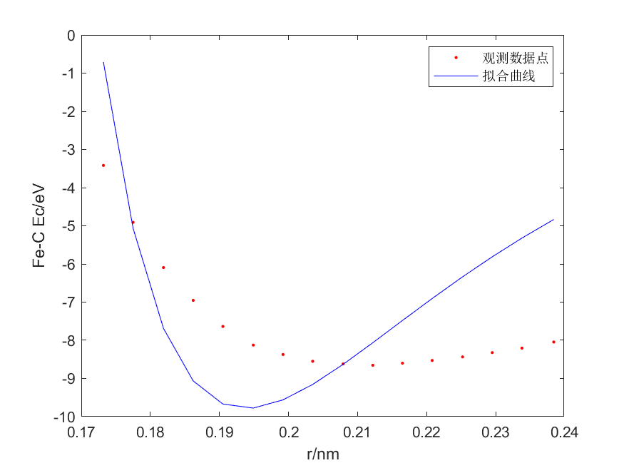
Fig 1. Lennard-Jones势函数拟合曲线

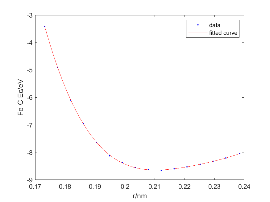
Fig 2. 傅里叶函数拟合曲线

3. Logistic曲线拟合

用MATLAB程序拟合Logistic函数：

$y=\frac{A}{1+Be^{-Ct}}$

MATLAB程序：

clear
clc
xdata=0:10:180;
ydata=[0 0 0.45 2.7 5.4 5.7 10.5 10.8 9.6 12.15 16.65 18.15 19.05 28.2 29.1 21.1 19.95 22.05 25.2];
%% 指定非线性函数拟合曲线
X0=[100 10 0.2];
[parameter,resnorm]=lsqcurvefit(@fun,X0,xdata,ydata); %指定拟合曲线
A=parameter(1);
B=parameter(2);
C=parameter(3);
fprintf('拟合Logistic曲线的参数A为：%.8f，B为：%.8f，C为：%.8f', A, B, C);
fit_y=fun(parameter,xdata);
figure(1)
plot(xdata, ydata, 'r*');
hold on
plot(xdata,fit_y,'b-');
xlabel('t');
ylabel('y');
legend('观测数据点','拟合曲线', 'Location', 'northwest');
saveas(gcf,sprintf('Logistic曲线.jpg'),'bmp');
%% Logistic函数
% y=A/(1+B*exp(-C*t))
function f=fun(X,t)
f=X(1)./(1+X(2).*exp(-X(3).*(t)));
end

结果：

拟合Logistic曲线的参数A为：24.81239102，B为：28.61794544，C为：0.04152321

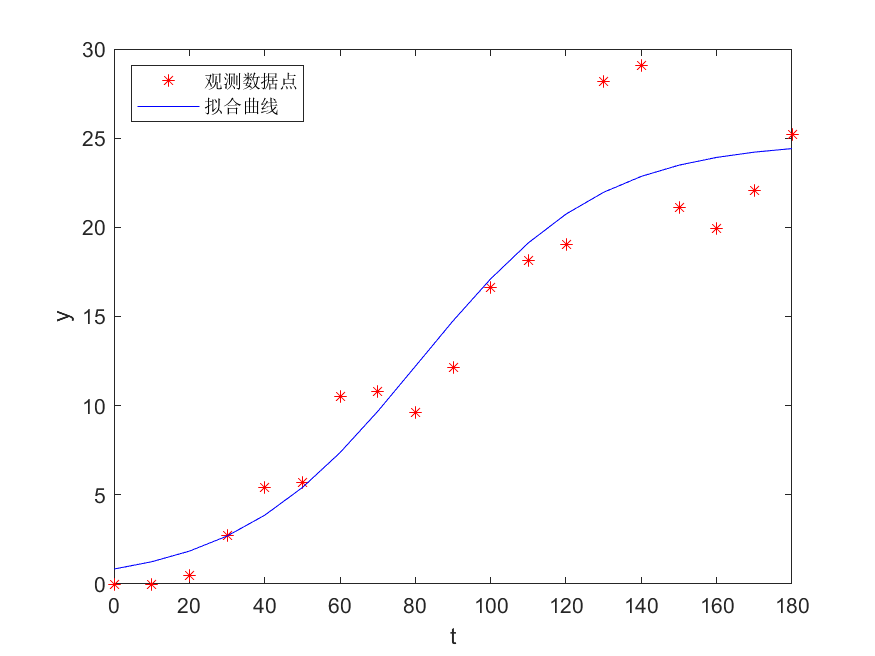
结果会受初始参数选取的影响。A是生长极限，初始取值时比y的最大值大一点。

注意：

多元非线性拟合请看：MATLAB实例：多元函数拟合(线性与非线性) - 凯鲁嘎吉 - 博客园

posted on 2019-11-12 08:30 凯鲁嘎吉阅读(8254) 评论(0) 编辑收藏举报