
密度峰值聚类算法(DPC)
凯鲁嘎吉 - 博客园 http://www.cnblogs.com/kailugaji/
具体实例见:密度峰值聚类算法MATLAB程序 - 凯鲁嘎吉 - 博客园
1. 简介
基于密度峰值的聚类算法全称为基于快速搜索和发现密度峰值的聚类算法(clustering by fast search and find of density peaks, DPC)。它是2014年在Science上提出的聚类算法,该算法能够自动地发现簇中心,实现任意形状数据的高效聚类。
该算法基于两个基本假设:1)簇中心(密度峰值点)的局部密度大于围绕它的邻居的局部密度;2)不同簇中心之间的距离相对较远。为了找到同时满足这两个条件的簇中心,该算法引入了局部密度的定义。
假设数据点 的局部密度为
 ,数据点
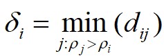
,数据点 到局部密度比它大且距离最近的数据点
 的距离为
的距离为 ,则有如下定义:
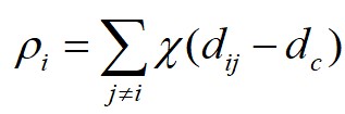
式中, 为
为 和
和 之间的距离;
 为截断距离;
 为逻辑判断函数,
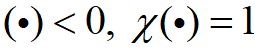 ,否则
,否则 。
。
这里对于局部密度最大的数据点 ,它的
,它的 。
。
根据以上定义,通过构造 相对于
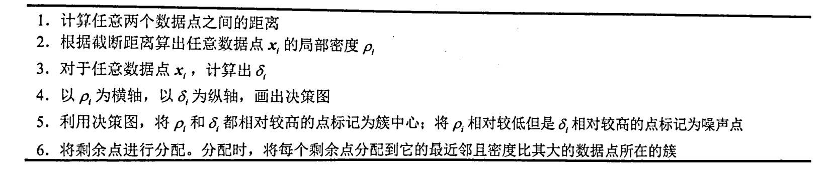
相对于 的决策图,进行数据点分配和噪声点剔除,可以快速得到最终的聚类结果。算法1给出了基于快速搜索和发现密度峰值的聚类算法的具体步骤。首先,基于快速搜索和发现密度峰值的聚类算法对任意两个数据点计算它们之间的距离,并依据截断距离计算出任意数据点
 的
的 和
和 ;然后,算法根据
 和
和 ,画出对应的聚类决策图;接着,算法利用得到的决策图,将
 和
和 都相对较高的数据点标记为簇的中心,将
 相对较低但是
 相对较高的点标记为噪声点;最后,算法将剩余的数据点进行分配,分配的规则为将每个剩余的数据点分配到它的最近邻且密度比其大的数据点所在的簇。
算法1 基于快速搜索和发现密度峰值的聚类算法
下面举一个简单的例子。在图1中,数据点的分布情况如图1(左)所示,可以看出数据集包含两个簇,分别用蓝色和红色标出,噪声用黑色标出。利用基于快速搜索和发现密度峰值算法,可以得到图1(右)的决策图。在决策过程中可以发现点1和点10的 和
和 都相对较高,因此它们被标记为中心点。点26~点28的
 相对较低但是
 相对较高,因此它们被标记为噪声。其他的点将被分配到它的最近邻且密度比其大的数据点所在的簇中去。
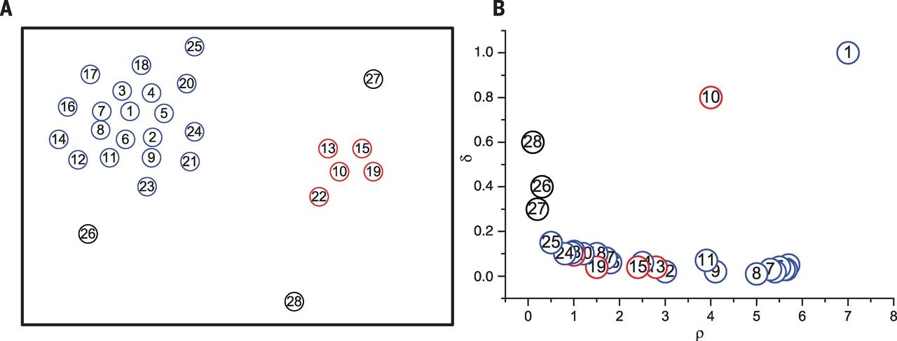
图1 基于快速搜索和发现密度峰值的聚类算法例子
基于快速搜索和发现密度峰值的聚类算法,想法非常直观,能够快速发现密度峰值点,并能够高效进行样本分配和发现噪声点。同时,因为该方法非常适用于大规模数据的聚类分析,因此具有很好的研究价值和应用前景。
2. MATLAB程序
数据请参考文献[3],也可以在这里下载:DPC数据.rar
clear all
close all
disp('The only input needed is a distance matrix file')
disp('The format of this file should be: ')
disp('Column 1: id of element i')
disp('Column 2: id of element j')
disp('Column 3: dist(i,j)')
%% 从文件中读取数据
mdist=input('name of the distance matrix file\n','s');
disp('Reading input distance matrix')
xx=load(mdist);
ND=max(xx(:,2));
NL=max(xx(:,1));
if (NL>ND)
  ND=NL; %% 确保 DN 取为第一二列最大值中的较大者,并将其作为数据点总数
end
N=size(xx,1); %% xx 第一个维度的长度,相当于文件的行数(即距离的总个数)

%% 初始化为零
for i=1:ND
  for j=1:ND
    dist(i,j)=0;
  end
end

%% 利用 xx 为 dist 数组赋值,注意输入只存了 0.5*DN(DN-1) 个值,这里将其补成了满矩阵
%% 这里不考虑对角线元素
for i=1:N
  ii=xx(i,1);
  jj=xx(i,2);
  dist(ii,jj)=xx(i,3);
  dist(jj,ii)=xx(i,3);
end

%% 确定 dc
percent=2.0;
fprintf('average percentage of neighbours (hard coded): %5.6f\n', percent);

position=round(N*percent/100);   %% round 是一个四舍五入函数
sda=sort(xx(:,3));   %% 对所有距离值作升序排列
dc=sda(position);

%% 计算局部密度 rho (利用 Gaussian 核)
fprintf('Computing Rho with gaussian kernel of radius: %12.6f\n', dc);

%% 将每个数据点的 rho 值初始化为零
for i=1:ND
  rho(i)=0.;
end

% Gaussian kernel
for i=1:ND-1
  for j=i+1:ND
     rho(i)=rho(i)+exp(-(dist(i,j)/dc)*(dist(i,j)/dc));
     rho(j)=rho(j)+exp(-(dist(i,j)/dc)*(dist(i,j)/dc));
  end
end
%
% "Cut off" kernel
%
%for i=1:ND-1
%  for j=i+1:ND
%    if (dist(i,j)<dc)
%       rho(i)=rho(i)+1.;
%       rho(j)=rho(j)+1.;
%    end
%  end
%end
%% 先求矩阵列最大值,再求最大值,最后得到所有距离值中的最大值
maxd=max(max(dist));
%% 将 rho 按降序排列,ordrho 保持序
[rho_sorted,ordrho]=sort(rho,'descend');
%% 处理 rho 值最大的数据点
delta(ordrho(1))=-1.;
nneigh(ordrho(1))=0;
%% 生成 delta 和 nneigh 数组
for ii=2:ND
   delta(ordrho(ii))=maxd;
   for jj=1:ii-1
     if(dist(ordrho(ii),ordrho(jj))<delta(ordrho(ii)))
        delta(ordrho(ii))=dist(ordrho(ii),ordrho(jj));
        nneigh(ordrho(ii))=ordrho(jj);
        % 记录 rho 值更大的数据点中与 ordrho(ii) 距离最近的点的编号 ordrho(jj)
     end
   end
end

%% 生成 rho 值最大数据点的 delta 值
delta(ordrho(1))=max(delta(:));

%% 决策图
disp('Generated file:DECISION GRAPH')
disp('column 1:Density')
disp('column 2:Delta')

fid = fopen('DECISION_GRAPH', 'w');
for i=1:ND
   fprintf(fid, '%6.2f %6.2f\n', rho(i),delta(i));
end

%% 选择一个围住类中心的矩形
disp('Select a rectangle enclosing cluster centers')

%% 每台计算机,句柄的根对象只有一个,就是屏幕,它的句柄总是 0
%% >> scrsz = get(0,'ScreenSize')
%% scrsz =
%%            1           1        1280         800
%% 1280 和 800 就是你设置的计算机的分辨率,scrsz(4) 就是 800,scrsz(3) 就是 1280
scrsz = get(0,'ScreenSize');

%% 人为指定一个位置
figure('Position',[6 72 scrsz(3)/4. scrsz(4)/1.3]);

%% ind 和 gamma 在后面并没有用到
for i=1:ND
  ind(i)=i;
  gamma(i)=rho(i)*delta(i);
end

%% 利用 rho 和 delta 画出一个所谓的“决策图”
subplot(2,1,1)
tt=plot(rho(:),delta(:),'o','MarkerSize',5,'MarkerFaceColor','k','MarkerEdgeColor','k');
title ('Decision Graph','FontSize',15.0)
xlabel ('\rho')
ylabel ('\delta')

fig=subplot(2,1,1);
rect = getrect(fig);

%% getrect 从图中用鼠标截取一个矩形区域, rect 中存放的是
%% 矩形左下角的坐标 (x,y) 以及所截矩形的宽度和高度
rhomin=rect(1);
deltamin=rect(2); %% 作者承认这是个 error,已由 4 改为 2 了!

%% 初始化 cluster 个数
NCLUST=0;

%% cl 为归属标志数组,cl(i)=j 表示第 i 号数据点归属于第 j 个 cluster
%% 先统一将 cl 初始化为 -1
for i=1:ND
  cl(i)=-1;
end

%% 在矩形区域内统计数据点(即聚类中心)的个数
for i=1:ND
  if ( (rho(i)>rhomin) && (delta(i)>deltamin))
     NCLUST=NCLUST+1;
     cl(i)=NCLUST;  %% 第 i 号数据点属于第 NCLUST 个 cluster
     icl(NCLUST)=i; %% 逆映射,第 NCLUST 个 cluster 的中心为第 i 号数据点
  end
end
fprintf('NUMBER OF CLUSTERS: %i \n', NCLUST);
disp('Performing assignation')

%assignation
%% 将其他数据点归类 (assignation)
for i=1:ND
  if (cl(ordrho(i))==-1)
    cl(ordrho(i))=cl(nneigh(ordrho(i)));
  end
end
%halo
%% 由于是按照 rho 值从大到小的顺序遍历,循环结束后, cl 应该都变成正的值了.

%% 处理光晕点,halo这段代码应该移到 if (NCLUST>1) 内去比较好吧
for i=1:ND
  halo(i)=cl(i);
end
if (NCLUST>1)
     % 初始化数组 bord_rho 为 0,每个 cluster 定义一个 bord_rho 值
  for i=1:NCLUST
    bord_rho(i)=0.;
  end
  % 获取每一个 cluster 中平均密度的一个界 bord_rho
  for i=1:ND-1
    for j=i+1:ND
        %% 距离足够小但不属于同一个 cluster 的 i 和 j
      if ((cl(i)~=cl(j))&& (dist(i,j)<=dc))
        rho_aver=(rho(i)+rho(j))/2.;  %% 取 i,j 两点的平均局部密度
        if (rho_aver>bord_rho(cl(i)))
          bord_rho(cl(i))=rho_aver;
        end
        if (rho_aver>bord_rho(cl(j)))
          bord_rho(cl(j))=rho_aver;
        end
      end
    end
  end

%% halo 值为 0 表示为 outlier
  for i=1:ND
    if (rho(i)<bord_rho(cl(i)))
      halo(i)=0;
    end
  end
end

%% 逐一处理每个 cluster
for i=1:NCLUST
  nc=0;  %% 用于累计当前 cluster 中数据点的个数
  nh=0;  %% 用于累计当前 cluster 中核心数据点的个数
  for j=1:ND
    if (cl(j)==i)
      nc=nc+1;
    end
    if (halo(j)==i)
      nh=nh+1;
    end
  end
  fprintf('CLUSTER: %i CENTER: %i ELEMENTS: %i CORE: %i HALO: %i \n', i,icl(i),nc,nh,nc-nh);
end

cmap=colormap;
for i=1:NCLUST
   ic=int8((i*64.)/(NCLUST*1.));
   subplot(2,1,1)
   hold on
   plot(rho(icl(i)),delta(icl(i)),'o','MarkerSize',8,'MarkerFaceColor',cmap(ic,:),'MarkerEdgeColor',cmap(ic,:));
end
subplot(2,1,2)
disp('Performing 2D nonclassical multidimensional scaling')
Y1 = mdscale(dist, 2, 'criterion','metricstress');
plot(Y1(:,1),Y1(:,2),'o','MarkerSize',2,'MarkerFaceColor','k','MarkerEdgeColor','k');
title ('2D Nonclassical multidimensional scaling','FontSize',15.0)
xlabel ('X')
ylabel ('Y')
for i=1:ND
 A(i,1)=0.;
 A(i,2)=0.;
end
for i=1:NCLUST
  nn=0;
  ic=int8((i*64.)/(NCLUST*1.));
  for j=1:ND
    if (halo(j)==i)
      nn=nn+1;
      A(nn,1)=Y1(j,1);
      A(nn,2)=Y1(j,2);
    end
  end
  hold on
  plot(A(1:nn,1),A(1:nn,2),'o','MarkerSize',2,'MarkerFaceColor',cmap(ic,:),'MarkerEdgeColor',cmap(ic,:));
end

%for i=1:ND
%   if (halo(i)>0)
%      ic=int8((halo(i)*64.)/(NCLUST*1.));
%      hold on
%      plot(Y1(i,1),Y1(i,2),'o','MarkerSize',2,'MarkerFaceColor',cmap(ic,:),'MarkerEdgeColor',cmap(ic,:));
%   end
%end
faa = fopen('CLUSTER_ASSIGNATION', 'w');
disp('Generated file:CLUSTER_ASSIGNATION')
disp('column 1:element id')
disp('column 2:cluster assignation without halo control')
disp('column 3:cluster assignation with halo control')
for i=1:ND
   fprintf(faa, '%i %i %i\n',i,cl(i),halo(i));
end
3. 结果
>> cluster_dp
The only input needed is a distance matrix file
The format of this file should be:
Column 1: id of element i
Column 2: id of element j
Column 3: dist(i,j)
name of the distance matrix file
example_distances.dat
Reading input distance matrix
average percentage of neighbours (hard coded): 2.000000
Computing Rho with gaussian kernel of radius:     0.033000
Generated file:DECISION GRAPH
column 1:Density
column 2:Delta
Select a rectangle enclosing cluster centers
NUMBER OF CLUSTERS: 5
Performing assignation
CLUSTER: 1 CENTER: 149 ELEMENTS: 378 CORE: 260 HALO: 118
CLUSTER: 2 CENTER: 451 ELEMENTS: 326 CORE: 250 HALO: 76
CLUSTER: 3 CENTER: 1310 ELEMENTS: 884 CORE: 785 HALO: 99
CLUSTER: 4 CENTER: 1349 ELEMENTS: 297 CORE: 208 HALO: 89
CLUSTER: 5 CENTER: 1579 ELEMENTS: 115 CORE: 115 HALO: 0
Performing 2D nonclassical multidimensional scaling
Generated file:CLUSTER_ASSIGNATION
column 1:element id
column 2:cluster assignation without halo control
column 3:cluster assignation with halo control
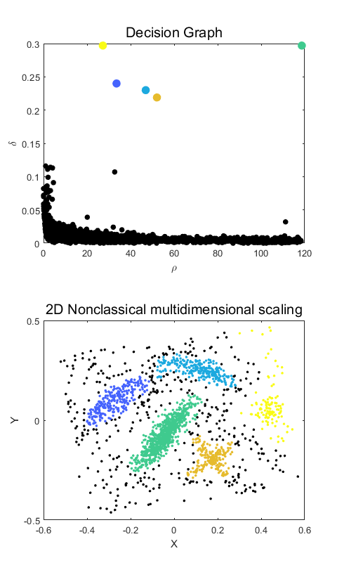
注:出错的话,将Y1 = mdscale(dist, 2, 'criterion','metricstress');换一个准则函数,比如改为Y1 = mdscale(dist, 2, 'criterion','sstress');
4. 参考文献
[1] Rodriguez A, Laio A. Clustering by fast search and find of density peaks [J]. Science, 2014, 344(6191): 1492-1496.
[2] 张宪超. 数据聚类. 北京:科学出版社, 2017.06.
[3] MATLAB程序:Clustering by fast search-and-find of density peaks
[4] 密度峰值聚类算法MATLAB程序

 浙公网安备 33010602011771号