利用sklearn对多分类的每个类别进行指标评价

  今天晚上，笔者接到客户的一个需要，那就是：对多分类结果的每个类别进行指标评价，也就是需要输出每个类型的精确率（precision），召回率（recall）以及F1值（F1-score）。
  对于这个需求，我们可以用sklearn来解决，方法并没有难，笔者在此仅做记录，供自己以后以及读者参考。
  我们模拟的数据如下：

y_true = ['北京', '上海', '成都', '成都', '上海', '北京', '上海', '成都', '北京', '上海']
y_pred = ['北京', '上海', '成都', '上海', '成都', '成都', '上海', '成都', '北京', '上海']

其中y_true为真实数据，y_pred为多分类后的模拟数据。使用sklearn.metrics中的classification_report即可实现对多分类的每个类别进行指标评价。
  示例的Python代码如下：

# -*- coding: utf-8 -*-
from sklearn.metrics import classification_report

y_true = ['北京', '上海', '成都', '成都', '上海', '北京', '上海', '成都', '北京', '上海']
y_pred = ['北京', '上海', '成都', '上海', '成都', '成都', '上海', '成都', '北京', '上海']

t = classification_report(y_true, y_pred, target_names=['北京', '上海', '成都'])

print(t)

输出结果如下：

              precision    recall  f1-score   support

          北京       0.75      0.75      0.75         4
          上海       1.00      0.67      0.80         3
          成都       0.50      0.67      0.57         3

    accuracy                           0.70        10
   macro avg       0.75      0.69      0.71        10
weighted avg       0.75      0.70      0.71        10

需要注意的是，输出的结果数据类型为str，如果需要使用该输出结果，则可将该方法中的output_dict参数设置为True，此时输出的结果如下:

{'北京': {'precision': 0.75, 'recall': 0.75, 'f1-score': 0.75, 'support': 4},
'上海': {'precision': 1.0, 'recall': 0.6666666666666666, 'f1-score': 0.8, 'support': 3},
'成都': {'precision': 0.5, 'recall': 0.6666666666666666, 'f1-score': 0.5714285714285715, 'support': 3},
'accuracy': 0.7,
'macro avg': {'precision': 0.75, 'recall': 0.6944444444444443, 'f1-score': 0.7071428571428572, 'support': 10},
'weighted avg': {'precision': 0.75, 'recall': 0.7, 'f1-score': 0.7114285714285715, 'support': 10}}

  使用confusion_matrix方法可以输出该多分类问题的混淆矩阵，代码如下：

from sklearn.metrics import confusion_matrix
y_true = ['北京', '上海', '成都', '成都', '上海', '北京', '上海', '成都', '北京', '上海']
y_pred = ['北京', '上海', '成都', '上海', '成都', '成都', '上海', '成都', '北京', '上海']
print(confusion_matrix(y_true, y_pred, labels = ['北京', '上海', '成都']))

输出结果如下：

[[2 0 1]
 [0 3 1]
 [0 1 2]]

  为了将该混淆矩阵绘制成图片，可使用如下的Python代码：

# -*- coding: utf-8 -*-
# author: Jclian91
# place: Daxing Beijing
# time: 2019-11-14 21:52

from sklearn.metrics import confusion_matrix
import matplotlib.pyplot as plt
import matplotlib as mpl

# 支持中文字体显示, 使用于Mac系统
zhfont=mpl.font_manager.FontProperties(fname="/Library/Fonts/Songti.ttc")

y_true = ['北京', '上海', '成都', '成都', '上海', '北京', '上海', '成都', '北京', '上海']
y_pred = ['北京', '上海', '成都', '上海', '成都', '成都', '上海', '成都', '北京', '上海']


classes = ['北京', '上海', '成都']
confusion = confusion_matrix(y_true, y_pred)

# 绘制热度图
plt.imshow(confusion, cmap=plt.cm.Greens)
indices = range(len(confusion))
plt.xticks(indices, classes, fontproperties=zhfont)
plt.yticks(indices, classes, fontproperties=zhfont)
plt.colorbar()
plt.xlabel('y_pred')
plt.ylabel('y_true')

# 显示数据
for first_index in range(len(confusion)):
    for second_index in range(len(confusion[first_index])):
        plt.text(first_index, second_index, confusion[first_index][second_index])

# 显示图片
plt.show()

生成的混淆矩阵图片如下：

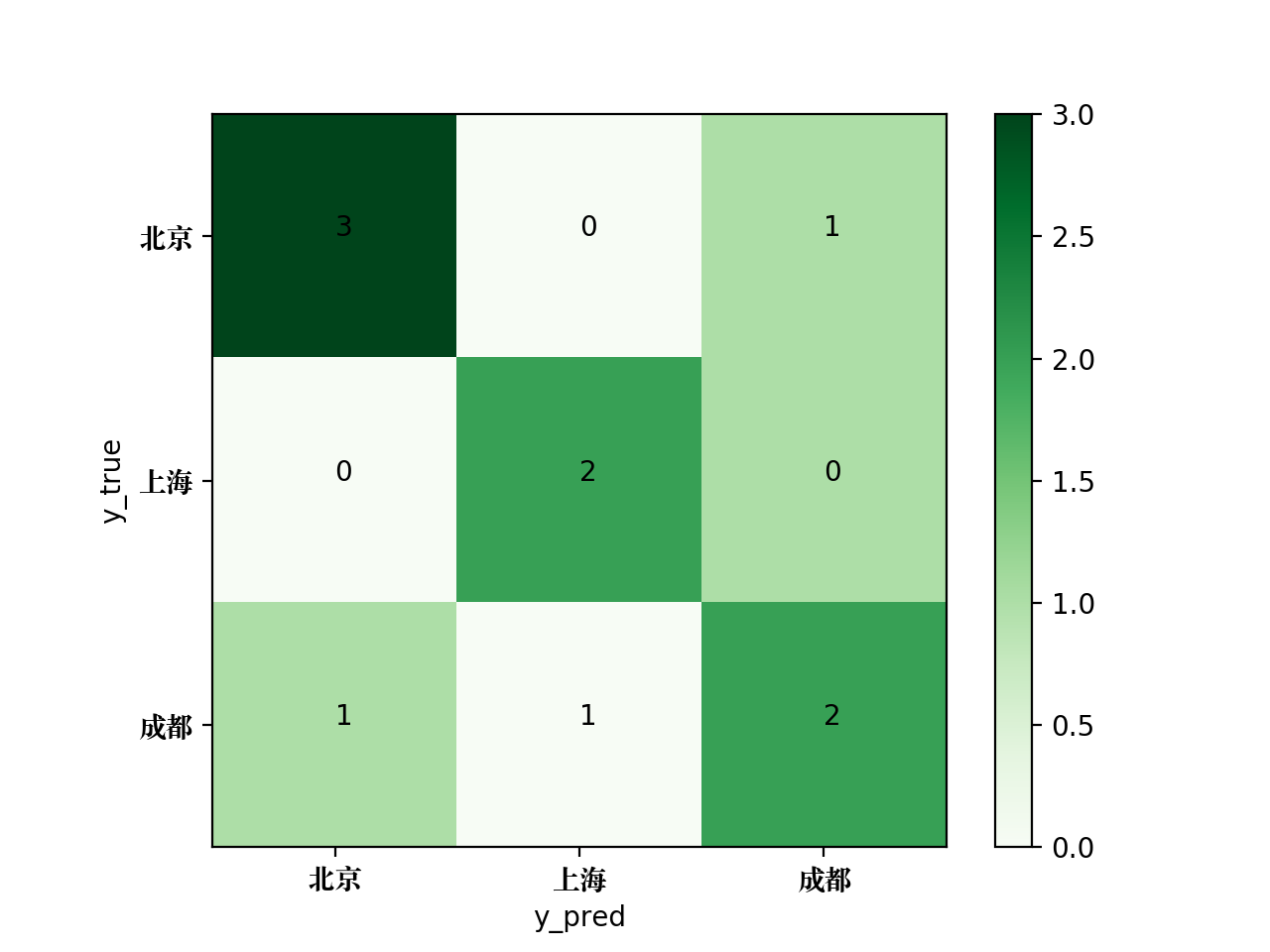
  本次分享到此结束，感谢大家阅读，也感谢在北京大兴待的这段日子，当然还会再待一阵子~