卷积神经网络 --- 网络可视化

 

卷积网络可视化

  深度学习可以从大量数据中提取有用的训练特征，但往往这些特征不具备可解释性，人们很能理解模型具体是如何进行学习的。对于卷积神经网络而言，其网络结构非常适合可视化，自2013年来，人们已经发展了许多技术来对网络训练过程进行解释和可视化，本文将重点介绍三种有效且常用的卷积神经网络可视化方法。对于第一种方法将使用猫狗分类的小型卷积神经网络，对于后两种可视化方法，将使用训练好的VGG16模型来进行演示。

可视化方法

中间激活

  可视化中间激活有助于理解卷积神经网络连续的层是如何对输入进行变换，也有助于更好的理解卷积神经网络每个过滤器的含义。

原理：

  可视化中间输出，指对于指定的输入，展示网络中各个卷积层和池化层输出的特征图。针对具体的输入，将从三个维度进行可视化：高度，宽度，通道数。每个通道往往对应着不同的特征，将每个通道内容绘制成二维图像，即可完成该目的的可视化。

应用方法：

  为了获得相应的特征图，需要先创建一个Keras模型，以测试图像作为输入，并输出所有的卷积层和池化层的激活。模型实例化需要有输入张量和输出张量，将特定输入映射为特定输出即得到最终的结果。

step1.导入训练模型

from keras.models import load_model

model = load_model('cats_and_dogs_small_2.h5')# 导入将要可视化的模型
model.summary()  # As a reminder.

step2.处理测试图像

# 图片地址
img_path = '/Users/fchollet/Downloads/cats_and_dogs_small/test/cats/cat.1700.jpg'

# We preprocess the image into a 4D tensor
from keras.preprocessing import image
import numpy as np

img = image.load_img(img_path, target_size=(150, 150))# 加载图片
img_tensor = image.img_to_array(img)# 将图片转换成张量形式
img_tensor = np.expand_dims(img_tensor, axis=0)# 将张量增维
# Remember that the model was trained on inputs
# that were preprocessed in the following way:
img_tensor /= 255. # 压缩到0-1

# Its shape is (1, 150, 150, 3)
print(img_tensor.shape)

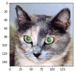
图1 原始图片

step3.模型实例化

from keras import models

# Extracts the outputs of the top 8 layers:
# 提取前八层输出
layer_outputs = [layer.output for layer in model.layers[:8]]
# Creates a model that will return these outputs, given the model input:
# 创建一个模型，给定输入返回输出
activation_model = models.Model(inputs=model.input, outputs=layer_outputs)

　#返回8个Numpy数组组成的列表，
　#每个层激活对应一个 Numpy 数组
　activations = activation_model.predict(img_tensor)

  first_layer_activation = activations[0]# 第一个卷积层的激活为148×148的特征图，有32个通道
  print(first_layer_activation.shape)

step4.测试结果

import matplotlib.pyplot as plt
# 可视化第三个通道
plt.matshow(first_layer_activation[0, :, :, 3], cmap='viridis')# 将矩阵或数组绘制成图像的函数
plt.show()

 

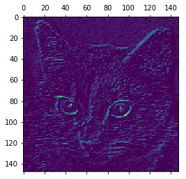
图2 中间激活可视化结果

过滤器

 

  可视化卷积神经网络中的过滤器可以更好的理解每个过滤器学习到的视觉模式。

原理：

  可视化过滤器可以通过在输入空间中进行梯度上升来实现：从空白输入图像开始，将梯度下降应用于卷积神经网络输入图像的值，来使某个过滤器的响应最大化。得到的图像是选定过滤器的最大响应图像。

应用方法：

step1.定义损失张量

from keras.applications import VGG16
from keras import backend as K

model = VGG16(weights='imagenet',# 导入VGG16作为模型
              include_top=False)

layer_name = 'block3_conv1'# 定义该层为可视化层
filter_index = 0# 定义可视化的过滤器

layer_output = model.get_layer(layer_name).output # 获得过滤器的输出
loss = K.mean(layer_output[:, :, :, filter_index])# 为过滤器定义损失张量

step2.获取损失相对于输入的梯度

grads = K.gradients(loss, model.input)[0]# 获取所示相对于输入的梯度

step3.通过随机梯度下降使损失最大化

# 给原始图像加噪
input_img_data = np.random.random((1, 150, 150, 3)) * 20 + 128.

step = 1.  # 每次梯度更新步长为 1
for i in range(40):
    loss_value, grads_value = iterate([input_img_data])# 计算损失值和梯度值
    input_img_data += grads_value * step# 沿着让损失最大化的方向调节输入图像

step4.将张量转换为有效图像的实用函数

# 将张量转换为有效图片
def deprocess_image(x):
    # normalize tensor: center on 0., ensure std is 0.1
    x -= x.mean()# 标准化处理，均值为0
    x /= (x.std() + 1e-5)# 标准差为0.1
    x *= 0.1

    # clip to [0, 1]
    x += 0.5
    x = np.clip(x, 0, 1)# 将张量裁剪到[0,1]

    # convert to RGB array
    x *= 255
    x = np.clip(x, 0, 255).astype('uint8')
    return x

step5.过滤器可视化

# 生成过滤器可视化函数
def generate_pattern(layer_name, filter_index, size=150):
    # Build a loss function that maximizes the activation
    # of the nth filter of the layer considered.
    layer_output = model.get_layer(layer_name).output
    loss = K.mean(layer_output[:, :, :, filter_index])

    # Compute the gradient of the input picture wrt this loss
    grads = K.gradients(loss, model.input)[0]

    # Normalization trick: we normalize the gradient
    grads /= (K.sqrt(K.mean(K.square(grads))) + 1e-5)

    # This function returns the loss and grads given the input picture
    iterate = K.function([model.input], [loss, grads])
    
    # We start from a gray image with some noise
    input_img_data = np.random.random((1, size, size, 3)) * 20 + 128.

    # Run gradient ascent for 40 steps
    step = 1.
    for i in range(40):
        loss_value, grads_value = iterate([input_img_data])
        input_img_data += grads_value * step
        
    img = input_img_data[0]
    return deprocess_image(img)

step6.生成某一层的可视化网格

for layer_name in ['block1_conv1', 'block2_conv1', 'block3_conv1', 'block4_conv1']:
    size = 64
    margin = 5

    # This a empty (black) image where we will store our results.
    results = np.zeros((8 * size + 7 * margin, 8 * size + 7 * margin, 3))# numpy数组来存放结果，结果与结果之间有黑色的边际

    for i in range(8):  # iterate over the rows of our results grid，行循环
        for j in range(8):  # iterate over the columns of our results grid，列循环
            # Generate the pattern for filter `i + (j * 8)` in `layer_name`
            filter_img = generate_pattern(layer_name, i + (j * 8), size=size)# 生成每个过滤器的可视化图

            # Put the result in the square `(i, j)` of the results grid
            horizontal_start = i * size + i * margin# 水平方向开始的调整
            horizontal_end = horizontal_start + size# 水平方向结束的调整
            vertical_start = j * size + j * margin# 垂直开始方向的调整
            vertical_end = vertical_start + size# 垂直结束方向的调整
            results[horizontal_start: horizontal_end, vertical_start: vertical_end, :] = filter_img# 最终所有过滤器的可视化结果

    # Display the results grid
    plt.figure(figsize=(20, 20))
    plt.imshow(results)
    plt.show()

 

图3 过滤器可视化结果

类激活热力图

  类激活热力图反映了训练图像的哪些部分对最终的分类决策起了重要作用。

原理：

  对给定的一张输入图像，对于一个卷积层的输出特征图，用类别相对于通道的梯度对这个特征图中的每个通道进行加权，简而言之，通过梯度的方法计算，每个通道得到的特征对类别的权重。

应用方法：

  这里将使用“Grad-CAM: visual explanations from deep networks via gradient-based localization”论文中介绍的方法。

step1.加载模型

from keras.applications.vgg16 import VGG16
# 加载带有预训练权重的 VGG16 网络
K.clear_session()

# Note that we are including the densely-connected classifier on top;
# all previous times, we were discarding it.
model = VGG16(weights='imagenet')

step2.处理输入图像

from keras.preprocessing import image
from keras.applications.vgg16 import preprocess_input, decode_predictions
import numpy as np

# The local path to our target image
img_path = '/Users/fchollet/Downloads/creative_commons_elephant.jpg'

# `img` is a PIL image of size 224x224
img = image.load_img(img_path, target_size=(224, 224))

# `x` is a float32 Numpy array of shape (224, 224, 3)
x = image.img_to_array(img)

# We add a dimension to transform our array into a "batch"
# of size (1, 224, 224, 3)
x = np.expand_dims(x, axis=0)# 增加一个维度，便于后续的计算

# Finally we preprocess the batch
# (this does channel-wise color normalization)
x = preprocess_input(x)# 按通道进行颜色标准化

 

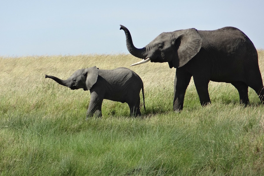
图4 原始图像

step3.应用Grad-CAM算法

african_elephant_output = model.output[:, 386]#预测向量中非洲象元素
last_conv_layer = model.get_layer('block5_conv3')#block5_conv3层的输出特征图，它是VGG16的最后一个卷积层
grads = K.gradients(african_elephant_output, last_conv_layer.output)[0]#“非洲象”类别相对于 block5_conv3输出特征图的梯度
pooled_grads = K.mean(grads, axis=(0, 1, 2))# 形状为(512,)的向量，每个元素是特定特征图通道的梯度平均大小
iterate = K.function([model.input], [pooled_grads, last_conv_layer.output[0]])# 访问刚刚定义的量，对于给定的样本图像pooled_grads和block_conv3层的输出特征图
pooled_grads_value, conv_layer_output_value = iterate([x])# 图像的numpy数组形式
# 将特征图组的每个通道乘以“该通道对大象类别的重要程度”

for i in range(512):
    conv_layer_output_value[:, :, i] *= pooled_grads_value[i]

heatmap = np.mean(conv_layer_output_value, axis=-1)#得到的特征图的逐通道平均值就是类激活热力图

step4.处理结果

# 使用Opencv来生成一张图像，将原始图像叠加在热力图上
import cv2

# 加载原图像
img = cv2.imread(img_path)

# 将热力图大小调整到与原图像相同
heatmap = cv2.resize(heatmap, (img.shape[1], img.shape[0]))

# 将热力图转换成RGB格式
heatmap = np.uint8(255 * heatmap)

# 将热力图应用于原始图像
heatmap = cv2.applyColorMap(heatmap, cv2.COLORMAP_JET)

# 0.4 为热力图强度因子
superimposed_img = heatmap * 0.4 + img

# 保存结果
cv2.imwrite('/Users/fchollet/Downloads/elephant_cam.jpg', superimposed_img)

 

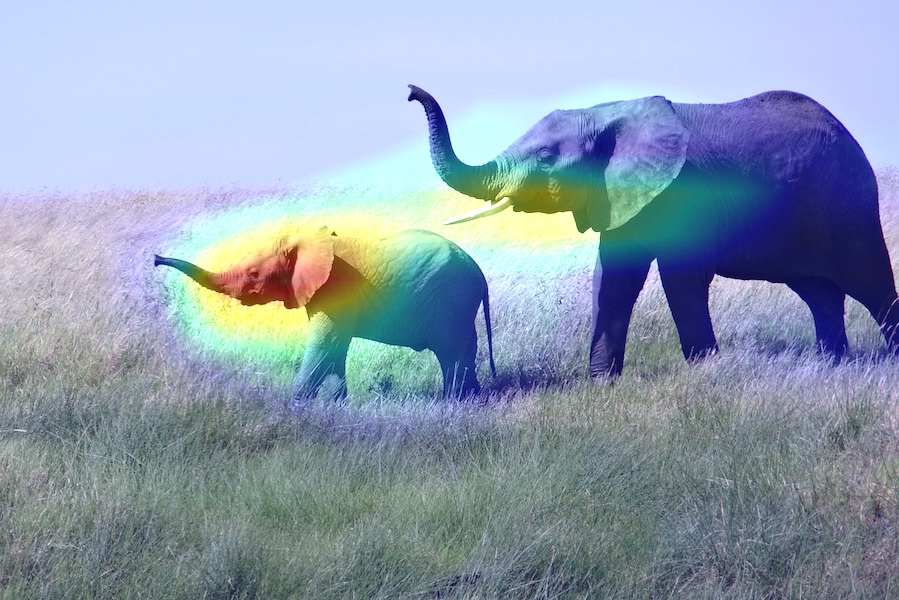
图5  类激活热力图