机器学习实战笔记(Python实现)-02-决策树
---------------------------------------------------------------------------------------
本系列文章为《机器学习实战》学习笔记,内容整理自书本,网络以及自己的理解,如有错误欢迎指正。
源码在Python3.5上测试均通过,代码及数据 --> https://github.com/Wellat/MLaction
---------------------------------------------------------------------------------------
1、算法概述及实现
1.1 算法理论
决策树构建的伪代码如下:

显然,决策树的生成是一个递归过程,在决策树基本算法中,有3种情导致递归返回:(1)当前结点包含的样本全属于同一类别,无需划分;(2)属性集为空,或是所有样本在所有属性上取值相同,无法划分;(3)当前结点包含的样本集合为空,不能划分。
划分选择
决策树学习的关键是第8行,即如何选择最优划分属性,一般而言,随着划分过程不断进行,我们希望决策树的分支节点所包含的样本尽可能属于同一类别,即结点的“纯度”越来越高。
①ID3算法
ID3算法通过对比选择不同特征下数据集的信息增益和香农熵来确定最优划分特征。
香农熵:
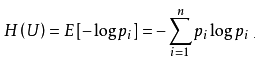
from collections import Counter
import operator
import math

def calcEnt(dataSet):
    classCount = Counter(sample[-1] for sample in dataSet)
    prob = [float(v)/sum(classCount.values()) for v in classCount.values()]
    return reduce(operator.add, map(lambda x: -x*math.log(x, 2), prob))
纯度差,也称为信息增益,表示为
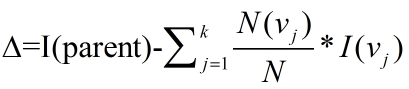
上面公式实际上就是当前节点的不纯度减去子节点不纯度的加权平均数,权重由子节点记录数与当前节点记录数的比例决定。信息增益越大,则意味着使用属性a来进行划分所获得的“纯度提升”越大,效果越好。
信息增益准则对可取值数目较多的属性有所偏好。
②C4.5算法
C4.5决策树生成算法相对于ID3算法的重要改进是使用信息增益率来选择节点属性。它克服了ID3算法存在的不足:ID3算法只适用于离散的描述属性,对于连续数据需离散化,而C4.5则离散连续均能处理。
增益率定义为:
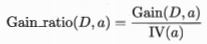
其中

需注意的是,增益率准则对可取值数目较少的属性有所偏好,因此,C4.5算法并不是直接选择增益率最大的候选划分属性,而是使用了一个启发式:先从候选划分属性中找出信息增益高于平均水平的属性,再从中选择增益率最高的。
③CART算法
CART决策树使用“基尼指数”来选择划分属性,数据集D的纯度可用基尼值来度量:

它反映了从数据集D中随机抽取两个样本,其类别标记不一致的概率。因此Gini(D)越小,则数据集D的纯度越高。
from  collections import Counter
import operator

def calcGini(dataSet):
    labelCounts = Counter(sample[-1] for sample in dataSet)
    prob = [float(v)/sum(labelCounts.values()) for v in labelCounts.values()]
    return 1 - reduce(operator.add, map(lambda x: x**2, prob))
剪枝处理
为避免过拟合,需要对生成树剪枝。决策树剪枝的基本策略有“预剪枝”和“后剪枝”。预剪枝是指在决策树生成过程中,对每个结点划分前先进行估计,若当前结点的划分不能带来决策树泛化性能提升,则停止划分并将当前结点标记为叶结点(有欠拟合风险)。后剪枝则是先从训练集生成一棵完整的决策树,然后自底向上地对非叶结点进行考察,若将该结点对应的子树替换为叶结点能带来决策树泛化性能提升,则将该子树替换为叶节点。
1.2 构造决策树
本书使用ID3算法划分数据集,即通过对比选择不同特征下数据集的信息增益和香农熵来确定最优划分特征。
1.2.1 计算香农熵:
 1 from math import log
 2 import operator
 3
 4 def createDataSet():
 5     '''
 6     产生测试数据
 7     '''
 8     dataSet = [[1, 1, 'yes'],
 9                [1, 1, 'yes'],
10                [1, 0, 'no'],
11                [0, 1, 'no'],
12                [0, 1, 'no']]
13     labels = ['no surfacing','flippers']
14     return dataSet, labels
15
16 def calcShannonEnt(dataSet):
17     '''
18     计算给定数据集的香农熵
19     '''
20     numEntries = len(dataSet)
21     labelCounts = {}
22     #统计每个类别出现的次数,保存在字典labelCounts中
23     for featVec in dataSet:
24         currentLabel = featVec[-1]
25         if currentLabel not in labelCounts.keys(): labelCounts[currentLabel] = 0
26         labelCounts[currentLabel] += 1 #如果当前键值不存在,则扩展字典并将当前键值加入字典
27     shannonEnt = 0.0
28     for key in labelCounts:
29         #使用所有类标签的发生频率计算类别出现的概率
30         prob = float(labelCounts[key])/numEntries
31         #用这个概率计算香农熵
32         shannonEnt -= prob * log(prob,2) #取2为底的对数
33     return shannonEnt
34
35 if __name__== "__main__":
36     '''
37     计算给定数据集的香农熵
38     '''
39     dataSet,labels = createDataSet()
40     shannonEnt = calcShannonEnt(dataSet)
1.2.2 划分数据集
 1 def splitDataSet(dataSet, axis, value):
 2     '''
 3     按照给定特征划分数据集
 4     dataSet:待划分的数据集
 5     axis:   划分数据集的第axis个特征
 6     value:  特征的返回值(比较值)
 7     '''
 8     retDataSet = []
 9     #遍历数据集中的每个元素,一旦发现符合要求的值,则将其添加到新创建的列表中
10     for featVec in dataSet:
11         if featVec[axis] == value:
12             reducedFeatVec = featVec[:axis]
13             reducedFeatVec.extend(featVec[axis+1:])
14             retDataSet.append(reducedFeatVec)
15             #extend()和append()方法功能相似,但在处理列表时,处理结果完全不同
16             #a=[1,2,3]  b=[4,5,6]
17             #a.append(b) = [1,2,3,[4,5,6]]
18             #a.extend(b) = [1,2,3,4,5,6]
19     return retDataSet
划分数据集的结果如下所示:
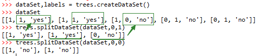
选择最好的数据集划分方式。接下来我们将遍历整个数据集,循环计算香农熵和 splitDataSet() 函数,找到最好的特征划分方式。
 1 def chooseBestFeatureToSplit(dataSet):
 2     '''
 3     选择最好的数据集划分方式
 4     输入:数据集
 5     输出:最优分类的特征的index
 6     '''
 7     #计算特征数量
 8     numFeatures = len(dataSet[0]) - 1
 9     baseEntropy = calcShannonEnt(dataSet)
10     bestInfoGain = 0.0; bestFeature = -1
11     for i in range(numFeatures):
12         #创建唯一的分类标签列表
13         featList = [example[i] for example in dataSet]
14         uniqueVals = set(featList)
15         #计算每种划分方式的信息熵
16         newEntropy = 0.0
17         for value in uniqueVals:
18             subDataSet = splitDataSet(dataSet, i, value)
19             prob = len(subDataSet)/float(len(dataSet))
20             newEntropy += prob * calcShannonEnt(subDataSet)
21         infoGain = baseEntropy - newEntropy
22         #计算最好的信息增益,即infoGain越大划分效果越好
23         if (infoGain > bestInfoGain):
24             bestInfoGain = infoGain
25             bestFeature = i
26     return bestFeature
1.2.3 递归构建决策树
目前我们已经学习了从数据集构造决策树算法所需要的子功能模块,其工作原理如下:得到原始数据集,然后基于最好的属性值划分数据集,由于特征值可能多于两个,因此可能存在大于两个分支的数据集划分。第一次划分之后,数据将被向下传递到树分支的下一个节点,在这个节点上,我们可以再次划分数据。因此我们可以采用递归的原则处理数据集。递归结束的条件是:程序遍历完所有划分数据集的属性,或者每个分支下的所有实例都具有相同的分类。
由于特征数目并不是在每次划分数据分组时都减少,因此这些算法在实际使用时可能引起一定的问题。目前我们并不需要考虑这个问题,只需要在算法开始运行前计算列的数目,查看算法是否使用了所有属性即可。如果数据集已经处理了所有属性,但是类标签依然不是唯一的,此时我们通常会采用多数表决的方法决定该叶子节点的分类。
在 trees.py 中增加如下投票表决代码:
 1 import operator
 2 def majorityCnt(classList):
 3     '''
 4     投票表决函数
 5     输入classList:标签集合,本例为:['yes', 'yes', 'no', 'no', 'no']
 6     输出:得票数最多的分类名称
 7     '''
 8     classCount={}
 9     for vote in classList:
10         if vote not in classCount.keys(): classCount[vote] = 0
11         classCount[vote] += 1
12     #把分类结果进行排序,然后返回得票数最多的分类结果
13     sortedClassCount = sorted(classCount.items(), key=operator.itemgetter(1), reverse=True)
14     return sortedClassCount[0][0]
创建树的函数代码(主函数):
 1 def createTree(dataSet,labels):
 2     '''
 3     创建树
 4     输入:数据集和标签列表
 5     输出:树的所有信息
 6     '''
 7     # classList为数据集的所有类标签
 8     classList = [example[-1] for example in dataSet]
 9     # 停止条件1:所有类标签完全相同,直接返回该类标签
10     if classList.count(classList[0]) == len(classList):
11         return classList[0]
12     # 停止条件2:遍历完所有特征时仍不能将数据集划分成仅包含唯一类别的分组,则返回出现次数最多的类标签
13     #
14     if len(dataSet[0]) == 1:
15         return majorityCnt(classList)
16     # 选择最优分类特征
17     bestFeat = chooseBestFeatureToSplit(dataSet)
18     bestFeatLabel = labels[bestFeat]
19     # myTree存储树的所有信息
20     myTree = {bestFeatLabel:{}}
21     # 以下得到列表包含的所有属性值
22     del(labels[bestFeat])
23     featValues = [example[bestFeat] for example in dataSet]
24     uniqueVals = set(featValues)
25     # 遍历当前选择特征包含的所有属性值
26     for value in uniqueVals:
27         subLabels = labels[:]
28         myTree[bestFeatLabel][value] = createTree(splitDataSet(dataSet, bestFeat, value),subLabels)
29     return myTree
本例返回 myTree 为字典类型,如下:
{'no surfacing': {0: 'no', 1: {'flippers': {0: 'no', 1: 'yes'}}}}
2、测试分类和存储分类器
利用决策树的分类函数:
 1 def classify(inputTree,featLabels,testVec):
 2     '''
 3     决策树的分类函数
 4     inputTree:训练好的树信息
 5     featLabels:标签列表
 6     testVec:测试向量
 7     '''
 8     # 在2.7中,找到key所对应的第一个元素为:firstStr = myTree.keys()[0],
 9     # 这在3.4中运行会报错:‘dict_keys‘ object does not support indexing,这是因为python3改变了dict.keys,
10     # 返回的是dict_keys对象,支持iterable 但不支持indexable,
11     # 我们可以将其明确的转化成list,则此项功能在3中应这样实现:
12     firstSides = list(inputTree.keys())
13     firstStr = firstSides[0]
14     secondDict = inputTree[firstStr]
15     # 将标签字符串转换成索引
16     featIndex = featLabels.index(firstStr)
17     key = testVec[featIndex]
18     valueOfFeat = secondDict[key]
19     # 递归遍历整棵树,比较testVec变量中的值与树节点的值,如果到达叶子节点,则返回当前节点的分类标签
20     if isinstance(valueOfFeat, dict):
21         classLabel = classify(valueOfFeat, featLabels, testVec)
22     else: classLabel = valueOfFeat
23     return classLabel
24
25 if __name__== "__main__":
26     '''
27     测试分类效果
28     '''
29     dataSet,labels = createDataSet()
30     myTree = createTree(dataSet,labels)
31     ans = classify(myTree,labels,[1,0])
决策树模型的存储
 1 def storeTree(inputTree,filename):
 2     '''
 3     使用pickle模块存储决策树
 4     '''
 5     import pickle
 6     fw = open(filename,'wb+')
 7     pickle.dump(inputTree,fw)
 8     fw.close()
 9
10 def grabTree(filename):
11     '''
12     导入决策树模型
13     '''
14     import pickle
15     fr = open(filename,'rb')
16     return pickle.load(fr)
17
18 if __name__== "__main__":
19     '''
20     存取操作
21     '''
22     storeTree(myTree,'mt.txt')
23     myTree2 = grabTree('mt.txt')
3、使用 Matplotlib 绘制树形图
上节我们已经学习如何从数据集中创建决策树,然而字典的表示形式非常不易于理解,决策树的主要优点就是直观易于理解,如果不能将其直观显示出来,就无法发挥其优势。本节使用 Matplotlib 库编写代码绘制决策树。
创建名为 treePlotter.py 的新文件:
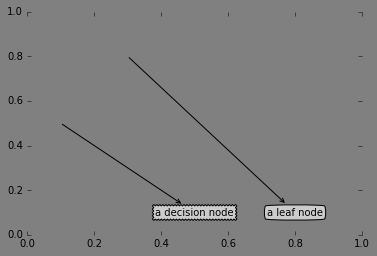
3.1 绘制树节点
 1 import matplotlib.pyplot as plt
 2
 3 # 定义文本框和箭头格式
 4 decisionNode = dict(boxstyle="sawtooth", fc="0.8")
 5 leafNode = dict(boxstyle="round4", fc="0.8")
 6 arrow_args = dict(arrowstyle="<-")
 7
 8 # 绘制带箭头的注释
 9 def plotNode(nodeTxt, centerPt, parentPt, nodeType):
10     createPlot.ax1.annotate(nodeTxt, xy=parentPt,  xycoords='axes fraction',
11              xytext=centerPt, textcoords='axes fraction',
12              va="center", ha="center", bbox=nodeType, arrowprops=arrow_args )
13
14 def createPlot():
15     fig = plt.figure(1, facecolor='grey')
16     fig.clf()
17     # 定义绘图区
18     createPlot.ax1 = plt.subplot(111, frameon=False) #ticks for demo puropses
19     plotNode('a decision node', (0.5, 0.1), (0.1, 0.5), decisionNode)
20     plotNode('a leaf node', (0.8, 0.1), (0.3, 0.8), leafNode)
21     plt.show()
22
23 if __name__== "__main__":
24     '''
25     绘制树节点
26     '''
27     createPlot()
结果如下:
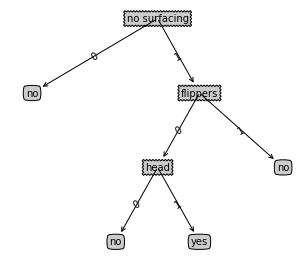
3.2 构造注解树
绘制一棵完整的树需要一些技巧。我们虽然有 x, y 坐标,但是如何放置所有的树节点却是个问题。我们必须知道有多少个叶节点,以便可以正确确x轴的长度;我们还需要知道树有多少层,来确定y轴的高度。这里另一两个新函数 getNumLeafs() 和 getTreeDepth() ,来获取叶节点的数目和树的层数,createPlot() 为主函数,完整代码如下:
  1 import matplotlib.pyplot as plt
  2
  3 # 定义文本框和箭头格式
  4 decisionNode = dict(boxstyle="sawtooth", fc="0.8")
  5 leafNode = dict(boxstyle="round4", fc="0.8")
  6 arrow_args = dict(arrowstyle="<-")
  7
  8 # 绘制带箭头的注释
  9 def plotNode(nodeTxt, centerPt, parentPt, nodeType):
 10     createPlot.ax1.annotate(nodeTxt, xy=parentPt,  xycoords='axes fraction',
 11              xytext=centerPt, textcoords='axes fraction',
 12              va="center", ha="center", bbox=nodeType, arrowprops=arrow_args )
 13
 14 def createPlot(inTree):
 15     '''
 16     绘树主函数
 17     '''
 18     fig = plt.figure(1, facecolor='white')
 19     fig.clf()
 20     # 设置坐标轴数据
 21     axprops = dict(xticks=[], yticks=[])
 22     # 无坐标轴
 23     createPlot.ax1 = plt.subplot(111, frameon=False, **axprops)
 24     # 带坐标轴
 25 #    createPlot.ax1 = plt.subplot(111, frameon=False)
 26     plotTree.totalW = float(getNumLeafs(inTree))
 27     plotTree.totalD = float(getTreeDepth(inTree))
 28     # 两个全局变量plotTree.xOff和plotTree.yOff追踪已经绘制的节点位置,
 29     # 以及放置下一个节点的恰当位置
 30     plotTree.xOff = -0.5/plotTree.totalW; plotTree.yOff = 1.0;
 31     plotTree(inTree, (0.5,1.0), '')
 32     plt.show()
 33
 34
 35 def getNumLeafs(myTree):
 36     '''
 37     获取叶节点的数目
 38     '''
 39     numLeafs = 0
 40     firstSides = list(myTree.keys())
 41     firstStr = firstSides[0]
 42     secondDict = myTree[firstStr]
 43     for key in secondDict.keys():
 44         # 判断节点是否为字典来以此判断是否为叶子节点
 45         if type(secondDict[key]).__name__=='dict':
 46             numLeafs += getNumLeafs(secondDict[key])
 47         else:   numLeafs +=1
 48     return numLeafs
 49
 50 def getTreeDepth(myTree):
 51     '''
 52     获取树的层数
 53     '''
 54     maxDepth = 0
 55     firstSides = list(myTree.keys())
 56     firstStr = firstSides[0]
 57     secondDict = myTree[firstStr]
 58     for key in secondDict.keys():
 59         if type(secondDict[key]).__name__=='dict':
 60             thisDepth = 1 + getTreeDepth(secondDict[key])
 61         else:   thisDepth = 1
 62         if thisDepth > maxDepth: maxDepth = thisDepth
 63     return maxDepth
 64
 65
 66 def plotMidText(cntrPt, parentPt, txtString):
 67     '''
 68     计算父节点和子节点的中间位置,并在此处添加简单的文本标签信息
 69     '''
 70     xMid = (parentPt[0]-cntrPt[0])/2.0 + cntrPt[0]
 71     yMid = (parentPt[1]-cntrPt[1])/2.0 + cntrPt[1]
 72     createPlot.ax1.text(xMid, yMid, txtString, va="center", ha="center", rotation=30)
 73
 74 def plotTree(myTree, parentPt, nodeTxt):#if the first key tells you what feat was split on
 75     # 计算宽与高
 76     numLeafs = getNumLeafs(myTree)  #this determines the x width of this tree
 77     depth = getTreeDepth(myTree)
 78     firstSides = list(myTree.keys())
 79     firstStr = firstSides[0]
 80     cntrPt = (plotTree.xOff + (1.0 + float(numLeafs))/2.0/plotTree.totalW, plotTree.yOff)
 81     # 标记子节点属性值
 82     plotMidText(cntrPt, parentPt, nodeTxt)
 83     plotNode(firstStr, cntrPt, parentPt, decisionNode)
 84     secondDict = myTree[firstStr]
 85     # 减少y偏移
 86     plotTree.yOff = plotTree.yOff - 1.0/plotTree.totalD
 87     for key in secondDict.keys():
 88         if type(secondDict[key]).__name__=='dict':#test to see if the nodes are dictonaires, if not they are leaf nodes
 89             plotTree(secondDict[key],cntrPt,str(key))        #recursion
 90         else:   #it's a leaf node print the leaf node
 91             plotTree.xOff = plotTree.xOff + 1.0/plotTree.totalW
 92             plotNode(secondDict[key], (plotTree.xOff, plotTree.yOff), cntrPt, leafNode)
 93             plotMidText((plotTree.xOff, plotTree.yOff), cntrPt, str(key))
 94     plotTree.yOff = plotTree.yOff + 1.0/plotTree.totalD
 95
 96
 97 def retrieveTree(i):
 98     '''
 99     保存了树的测试数据
100     '''
101     listOfTrees =[{'no surfacing': {0: 'no', 1: {'flippers': {0: 'no', 1: 'yes'}}}},
102                   {'no surfacing': {0: 'no', 1: {'flippers': {0: {'head': {0: 'no', 1: 'yes'}}, 1: 'no'}}}}
103                   ]
104     return listOfTrees[i]
105
106
107
108 if __name__== "__main__":
109     '''
110     绘制树
111     '''
112     createPlot(retrieveTree(1))
测试结果:
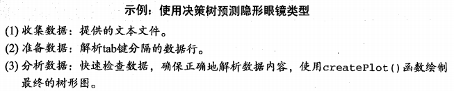
4、实例:使用决策树预测隐形眼镜类型
4.1 处理流程

数据格式如下所示,其中最后一列表示类标签:
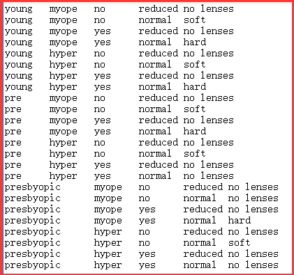
4.2 Python实现代码
1 import trees
2 import treePlotter
3
4 fr = open('lenses.txt')
5 lenses = [inst.strip().split('\t') for inst in fr.readlines()]
6 lensesLabels=['age','prescript','astigmatic','tearRate']
7 lensesTree = trees.createTree(lenses,lensesLabels)
8 treePlotter.createPlot(lensesTree)
产生的决策树:
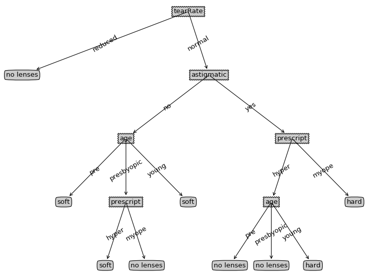
本节使用的算法成为ID3,它是一个号的算法但无法直接处理数值型数据,尽管我们可以通过量化的方法将数值型数据转化为标称型数值,但如果存在太多的特征划分,ID3算法仍然会面临其他问题。

 浙公网安备 33010602011771号