Plot函数用法详解——R语言

plot是R中的基本画图工具，直接plot(x)，x为一个数据集，就能画出图，soeasy！但是细节往往制胜的关键，所以就详细来看看plot的所有可设置参数及参数设置方法。R语言的基础绘图系统主要由基础包graphics提供，它包含了各式的图形绘制函数，如折线图、直方图、箱形图等，这里主要介绍plot()函数的用法，它主要用于绘制散点图和折线图。

一、plot函数用法

plot（）是常见的作图函数，其中的参数是需要熟悉的，以便在作图过程中更加灵活的处理图形的元素。

plot(x, y = NULL, type = "p", xlim = NULL, ylim = NULL, log = "", main = NULL, sub = NULL, xlab = NULL, ylab = NULL, ann = par("ann"), axes = TRUE, frame.plot = axes, panel.first = NULL, panel.last = NULL, asp = NA, xgap.axis = NA, ygap.axis = NA,   ...)

• x相当于自变量，y相当于因变量；
• y没缺省时，必须和x同长度，类型是可以向量化的数据结构，如向量、矩阵的行或列、数组的元素、数据框的列、列表的元素等；
• y缺省时，x为单列时，y默认为c(1:n)，其中n为x的长度；
• y缺省时，x为两列的矩阵或数据框，则该矩阵或数据框的第一、二列分别对应自变量和因变量。

Arguments

参数	描述
x,y	the x and y arguments provide the x and y coordinates for the plot. Any reasonable way of defining the coordinates is acceptable
type	character string giving the type of plot desired. The following values are possible
pch	a vector of plotting characters or symbols: see points
main	a main title for the plot, see also title
sub	Sub-title (at bottom) using font, size and color par(c("font.sub", "cex.sub", "col.sub"))
xlab ylab	a label for the x axis, defaults to a description of x, y
col	the foreground color of symbols as well as lines 用于指定颜色的参数,默认的绘图颜色。某些函数（如lines和pie）可以接受一个含有颜色值的向量并自动循环使用
cex	a numerical vector giving the amount by which plotting charactersand symbols should be scaled relative to the default
lty	用于线条类型的定义，指定值为整数，lty="1" lty="0"显示为空白，即无线条； lty="1"显示为实线线条；lty="2"显示为虚线线条；lty="3"显示为点状线条 等

二、plot参数精解

plot函数是一个泛型函数，是R基础绘图中的高级函数，不仅在一般图形绘制中需要用到，在模型的可视化也会用的，这里将Plot()常见的参数做一个讲解。

2.1 type参数设置绘图类型

参数	说明
"p" for points	散点图 默认
"l" for lines	线图
"b" for both	描点连线，点与线不相连
"c" for the lines part alone of "b"	线图，点空白
"o" for both ‘overplotted’	描点连线，线穿过点
"h" for ‘histogram’ like (or ‘high-density’) vertical lines	从0出发的垂线
"s" for stair steps	阶梯图
"S" for other steps, see ‘Details’ below
"n" for no plotting	空白图，只生成适合的横纵坐标轴

dev.off()
par(mfrow=c(2,4))   #2行4列
mtcars<-mtcars[order(mtcars$wt),]
plot(mtcars$wt,mtcars$disp,type='p',main="type='p'")
plot(mtcars$wt,mtcars$disp,type='l',main="type='l'")
plot(mtcars$wt,mtcars$disp,type='b',main="type='b'")
plot(mtcars$wt,mtcars$disp,type='c',main="type='c'")
plot(mtcars$wt,mtcars$disp,type='o',main="type='o'")
plot(mtcars$wt,mtcars$disp,type='h',main="type='h'")
plot(mtcars$wt,mtcars$disp,type='s',main="type='s'")
plot(mtcars$wt,mtcars$disp,type='S',main="type='S'")

2.2 pch参数设置点符号符号类型

plot函数中还有个pch参数是控制点的类型的，取值意义如下:

dev.off()
par(mfrow=c(2,4))#2行4列
plot(mtcars$wt,mtcars$disp,pch=1,main="pch=1")
plot(mtcars$wt,mtcars$disp,pch=3,main="pch=3")
plot(mtcars$wt,mtcars$disp,pch=5,main="pch=5")
plot(mtcars$wt,mtcars$disp,pch=7,main="pch=7")
plot(mtcars$wt,mtcars$disp,pch=9,main="pch=9")
plot(mtcars$wt,mtcars$disp,pch=11,main="pch=11")
plot(mtcars$wt,mtcars$disp,pch=13,main="pch=13")
plot(mtcars$wt,mtcars$disp,pch=15,main="pch=15")

2.3 lty参数设置线条类型

dev.off()
par(mfrow=c(2,3))
plot(mtcars$wt,mtcars$disp,type='l',lty=1,lwd=2,main="lty=1")
plot(mtcars$wt,mtcars$disp,type='l',lty=2,lwd=2,main="lty=2")
plot(mtcars$wt,mtcars$disp,type='l',lty=3,lwd=2,main="lty=3")
plot(mtcars$wt,mtcars$disp,type='l',lty=4,lwd=2,main="lty=4")
plot(mtcars$wt,mtcars$disp,type='l',lty=5,lwd=2,main="lty=5")
plot(mtcars$wt,mtcars$disp,type='l',lty=6,lwd=2,main="lty=6")

三、plot作图图例legend操作

Graphics包中与plot函数配套的一些低级绘图函数

函数	描述
abline	为图形添加截距为a、斜率为b的直线
arrows	在坐标点（x0,y0）和（x1,y1）之间绘制线段，并在端点处添加箭头
box	绘制图形的边框
layout	布局图形页面
legend	在坐标点（x,y）处添加图例
lines	在坐标点（x,y）之间添加直线
mtext	在图形区域的边距或区域的外部边距添加文本
points	在坐标点（x,y）处添加点
polygon	沿着坐标点（x,y）绘制多边形
polypath	绘制由一个或多个连接坐标点的路径组成的多边形
resterimaga	绘制一个或多个网络图像
rect	绘制一个左下角在（xleft,ybottom）处、右下角在（xright,ytop）处的矩形
rug	添加地毯图
segments	在坐标点（x0,y0）和（x1,y1）之间绘制线段
text	在坐标点（x,y）处添加文本
title	为图形添加标题
xspline	根据控制点（x,y）绘制x样条曲线（平滑曲线）

我们在一个图中画多组对象的时候，这个时候就需要图例来帮助我们读图，比如对下面的图，这个图中有两组数据，但却没有图例，我们不知道三角形和圈圈代表谁：

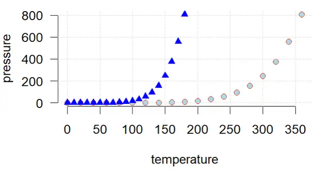
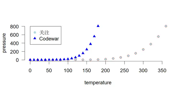
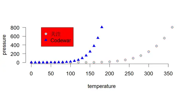
我们想加一个图例，这个时候就需要继续运行legend函数，比如我想圈圈代表‘关注’，三角代表‘Codewar’，这样就可以写出如下代码，这儿的“关注”和“Codewar”你都可以换成你想的任何字符哈，这里仅用它举例：

legend(0,800,
       c("关注","Codewar"), pch=c(19,17), col=c("lightblue","blue"))

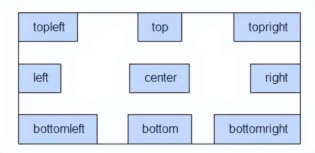
图例当然也可以改，首先就是改位置，位置的关键字有9个，对应的位置如下图：

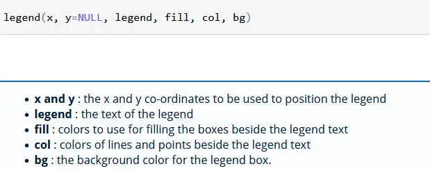
图例的位置可以用关键字改，也可以更加的个性化，用坐标改也是可以的，其可以接受的参数如下图：

比如想将原来的图例换成红色的背景，然后放在（25，800）这个坐标上，注意这个坐标与已画的图形相匹配，依据的是所做图的位置坐标，是相对数！！！，就可以写出如下代码：

legend(25,800,
       bg = 'red',
       c("关注","Codewar"), pch=c(19,17), col=c("lightblue","blue"))

运行后得到下图：

大家可以看到一个红色背景的图例已经在对应位置加上了，但是仔细观察上图，其实我们现在图是没有边框的，这个时候图例加个边框也不合适，所以我还想设置下图例的边框，甚至我还想改图例中的字体，甚至图例整体的大小，甚至是....统统都是可以的哈，就是这么牛！比如，我现在突发奇想，我想给我的图例加一个标题，再将其变小一点，放在右下角，并且让图例中的字水平排列，我就可以写出如下代码：

legend("bottomright", title="欢迎大家",
       c("关注","Codewar"),col=c("lightblue","blue"), horiz=TRUE, cex=0.4,
       box.lty=0,
       bg = 'red',
       text.font=4
       )

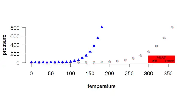
依然是给大家解释下上面代码中各个参数的意思：bottomright是图例位置的关键字，title是标题字符，horiz是图例内容水平排列，cex是图例整体大小，box.lty是图例边框（取0就是无框），text.font是字体（取4就是斜体）。

四、plot作图示例

4.1 例1

plot(mtcars)

4.2 例2

par(mfrow=c(1,1), mai=c(0.7, 0.7, 0.4, 0.4), cex=0.8)
set.seed(1)
x <- rnorm(200)      #产生200个服从正态分布的随机数 
y <- 1+2*x+rnorm(200)
d <- data.frame(x, y)
plot(x, y)   # 绘制散点图
#综合定制示例
plot(x, y, xlab='x=自变量', ylab='y=因变量')  # 添加坐标轴标题
grid(col='grey60')                            # 添加网格线
axis(side=4, col.ticks='blue', lty=1)         # 绘制坐标轴
polygon(d[chull(d),], lty=6, lwd=1, col='lightgreen') # 添加多边形
points(d)                                     # 重新绘制散点图
points(mean(x), mean(y), pch=19, cex=5, col=2)# 添加均值点
abline(v=mean(x), h=mean(y), lty=2, col='gray30') # 添加均值水平线和垂直线
abline(lm(y~x), lwd=2, col=2)                 # 添加回归直线
lines(lowess(y~x, f=1/6), col=4, lwd=2, lty=6)# 添加拟合曲线
segments(-0.8, 0, -1.6, 3.3, lty=6, col='blue')# 添加线段
arrows(0.45, -2.2, -0.8, -0.6, code=2, angle=25, length=0.06, col=2) 
# 添加带箭头的线段
text(-2.2, 3.5, labels=expression('拟合的曲线'), adj=c(-0.1, -0.02),col=4) 
# 添加注释文本
rect(0.4, -1.6, 1.6, -3.5, col='pink', border='grey60') # 添加矩形
mtext(expression(hat(y)==hat(beta)[0]+hat(beta)[1]*x), cex=0.9, side=1,
      line=-5.3, adj=0.72)                    # 添加注释表达式
legend('topleft', legend=c('拟合的直线', '拟合的曲线'), lty=c(1, 6), 
       col=c(2, 4), cex=0.8, fill=c('red', 'blue'), box.col='grey60',
       ncol=1, inset=0.02)                    # 添加图例
title('散点图及拟合直线和曲线\n并为图形添加新的元素', 
      cex.main=0.8, font.main=4)              # 添加标题并换行，使用斜体字
box(col=4, lwd=2)                             # 添加边框 

总结

R语言以其精美的图形而著称，它具有丰富的函数集，可用于构建和格式化任何种类的图形以及plot（）功能家族之一，可以帮助我们构建这些家族。用R语言画图，plot函数的使用频率应该是最高了，灵活运用会添光添彩。这些参数即可以在plot()中设置，也可以在一些依赖于plot()函数才能生效的其他函数中进行设置，最后都作用于plot()绘制的图形。

参考文献

R语言绘图基础教程
R语言(4) plot函数介绍
R语言绘图基础教程
R可视化：plot函数基础操作，小白教程
R语言绘图基础